
Disclaimer: This Jupyter Notebook contains content generated with the assistance of AI. While every effort has been made to review and validate the outputs, users should independently verify critical information before relying on it. The SELENE notebook repository is constantly evolving. We recommend downloading or pulling the latest version of this notebook from Github.
Apriori Algorithm (Association Rule Mining)
Association Rule Mining (ARM) is a fundamental data mining technique for discovering relationships among items that frequently occur together in transactional data. One of the most influential and widely used algorithms for this task is the Apriori algorithm, which introduced an efficient strategy for identifying frequent itemsets and generating association rules. Although many algorithms have since been proposed to improve performance under specific conditions, Apriori remains the standard algorithm for teaching the core principles of association rule mining because of its simplicity, interpretability, and historical significance.
The primary focus of the Apriori algorithm is the discovery of frequent itemsets, that is, sets of items whose occurrence frequency exceeds a user-defined minimum support threshold. This step is computationally the most expensive part of association rule mining because the number of possible itemsets grows exponentially with the number of distinct items. Apriori addresses this challenge by exploiting the Apriori property, which states that every subset of a frequent itemset must also be frequent. This property enables the algorithm to prune large portions of the search space, making the mining process significantly more efficient.
To provide a deeper understanding of how Apriori works, this notebook includes a from-scratch implementation of the algorithm using Python. Rather than relying on existing data mining libraries, each step of the algorithm (from candidate itemset generation and support counting to pruning based on minimum support) is implemented explicitly. This approach makes the underlying logic transparent and helps illustrate how the algorithm systematically reduces the search space while identifying frequent itemsets.
Understanding the Apriori algorithm is important because it introduces several fundamental concepts that extend far beyond association rule mining. The ideas of candidate generation, search space pruning, and exploiting monotonicity properties are widely used in data mining, machine learning, and combinatorial optimization. Moreover, learning how Apriori operates provides valuable insight into the computational challenges of pattern discovery and serves as a strong foundation for understanding more advanced frequent pattern mining algorithms, such as FP-Growth and ECLAT.
Setting up the Notebook
Make Required Imports
This notebook requires the import of different Python packages but also additional Python modules that are part of the repository. If a package is missing, use your preferred package manager (e.g., conda or pip) to install it. If the code cell below runs with any errors, all required packages and modules have successfully been imported.
from src.utils.helpers.arm import *
To provide some example code using existing and mature implementations of the Apriori algorithm, also import the efficient-apriori library. This library is not crucial for the purpose of this notebook, only some example code will not work without it.
from efficient_apriori import apriori
Preliminaries
- Although the notebook starts with a brief recap about Association Rule Mining, being already somewhat familiar with this data mining is recommended.
- The from-scratch implementation of the Apriori algorithm is for educational purposes and not suitable to find association rules in large, real-world datasets; you should use mature libraries for that.
Quick Recap: Association Rule Mining
Association Rule Mining (ARM) aims to discover interesting co-occurrence patterns among items in a collection of transactions, where each transaction is represented as a set of items (e.g., products purchased together in a shopping basket). The goal is to identify relationships that reveal how the presence of certain items is associated with the presence of others, enabling the extraction of meaningful rules such as "customers who buy bread and butter also tend to buy milk". These patterns provide valuable insights for decision-making in applications such as market basket analysis, recommendation systems, inventory management, and customer behavior analysis.
Basic Setup & Applications
ARM assumes that the data consist of a collection of transactions, where each transaction is represented as an unordered set of items. Let $I = \{i_1, i_2, \ldots, i_m\}$ denote the universal set of all possible items. A transaction database is then a collection of transactions $D = \{T_1, T_2, \ldots, T_n\}$, where each transaction $T_k$ is a subset of $I$ (i.e., $T_k \subseteq I$). In the classical market basket setting, each transaction corresponds to a customer's purchase, and the items are the products included in that purchase. More generally, a transaction may represent any observation that can be described as a collection of discrete items, such as visited web pages, diagnosed symptoms, or expressed genes.
The goal of ARM is to discover meaningful relationships or co-occurrence patterns among items in large datasets. Given a collection of transactions it identifies rules of the form $X \rightarrow Y$, indicating that when a set of items $X$ appears, another set of items $X$ is also likely to appear; $X$ and $Y$ are disjoint sets of items, i.e., $X, Y \subseteq I$ and $X\cap Y = \emptyset$. The right-hand side $X$ is called the $antecedent$; the left-hand side $Y$ is called the consequent The objective is not to establish causation, but to uncover associations that occur more frequently than expected by chance and may be useful for understanding the data or making decisions.
Association rule mining is most widely known for its application to Market Basket Analysis, where the objective is to discover products that customers frequently purchase together. This application popularized the field through examples such as identifying that customers who buy bread and butter are also likely to buy milk, enabling retailers to improve product placement, promotions, and recommendation systems. Because of its intuitive interpretation and commercial value, market basket analysis remains the canonical example used to introduce association rule mining.
However, the underlying methodology is much more general and can be applied to any dataset that can be represented as a collection of transactions, where each transaction is a set of discrete items. In each of these applications, the meaning of a "transaction" and an "item" changes, but the goal remains the same: to discover meaningful patterns of co-occurrence that reveal relationships among items and provide actionable insights.
Beyond market basket analysis, Association Rule Mining (ARM) has a wide range of applications across different domains where discovering relationships among co-occurring items or events is valuable. In healthcare, ARM is used to identify associations between diseases, symptoms, and treatments to support clinical decision-making. In web usage mining, it uncovers patterns in user navigation behavior to improve website design and personalize content. Recommendation systems leverage ARM to suggest products, movies, or music based on users' previous interactions. In cybersecurity, it helps detect suspicious activity by identifying unusual combinations of events associated with security breaches. ARM is also applied in bioinformatics to discover relationships among genes and proteins, in telecommunications to analyze network alarms and failures, and in fraud detection to reveal patterns of fraudulent transactions, demonstrating its versatility in extracting actionable knowledge from large transactional datasets.
Throughout this notebook, we introduce ARM in the context of Market Basket Analysis. More specifically, to keep it simple, we consider a very small set of items (i.e., supermarket products) $I = \{\text{bread}, \text{cereal}, \text{cheese}, \text{eggs}, \text{milk}, \text{yogurt}\}$ and the following set of $5$ transactions:
| ID | Items |
|---|---|
| 1 | bread, yogurt |
| 2 | bread, cereal, eggs, milk |
| 3 | cereal, cheese, milk, yogurt |
| 4 | bread, cereal, milk, yogurt |
| 5 | bread, cheese, milk, yogurt |
Important: Recall that basic ARM represents each transaction as a set of items, meaning that only the presence or absence of each item is considered. Consequently, the model ignores both the order of items and their multiplicity within a transaction. In the context of Market Basket Analysis, for example, a transaction containing the item "eggs" simply indicates that eggs were purchased, regardless of whether the customer bought a carton of 6 eggs, a dozen eggs, or several cartons. Likewise, if a customer purchases multiple units of the same product, the item appears only once in the transaction. Thus, basic association rule mining treats all transactions containing "eggs" identically, regardless of the quantity purchased, focusing solely on which items co-occur rather than how many units of each item are present.
Since we later implement the Apriori algorithm from scratch, let's define this simple transaction database as a Python list of transactions. Note that each transaction is represented as a tuple and not as a set. This is only for convenience and readability to allow all items in a transaction to be lexicographically sorted. Keep in mind that transactions are considered sets of items.
db = [
    ('bread', 'yogurt'),
    ('bread', 'cereal', 'eggs', 'milk'),
    ('cereal', 'cheese', 'milk', 'yogurt'),
    ('bread', 'cereal', 'milk', 'yogurt'),
    ('bread', 'cheese', 'milk', 'yogurt')
]
What are "Interesting" Rules?
Intuitively, an association rule expresses that when one set of items or events occurs, another item or set of items is likely to occur as well. For example, given our small Market Basket analysis dataset:
means that customers who buy cereal often also buy milk. In other words, an association rule captures a recurring co-occurrence pattern in the data, indicating that the presence of the left-hand side makes the right-hand side more likely, without implying causation or certainty.
Although any rule of the form $X \rightarrow Y$ can be considered an association rule, not every rule is useful or interesting. Many rules may describe coincidences, involve very rare items, or express relationships that are already expected (e.g., because $Y$ is very common). Such rules provide little actionable insight. What makes a rule "interesting" depends on the application and your goals. For example, a retailer may value rules that reveal profitable cross-selling opportunities, while a medical researcher may be interested in rare but highly reliable associations. Because there is no universal notion of interestingness, different evaluation measures are used to assess rules from different perspectives, including frequency, reliability, and the strength of the association.
We will introduce the most important and common evaluation metrics later more formally.
Naive ARM Algorithm
Let's assume that we have some evaluation measures that take in an association rule $X \rightarrow Y$ and return some numerical scores; again, covered later. Since the the set of items $I$ is finite, we can implement are very simple algorithm to find all interesting association rules
Generate all possible rules $X \rightarrow Y$ with $X, Y \subseteq I$ and $X\cap Y = \emptyset$
For each rule, check if it qualifies with respect to the evaluation metrics (i.e., if the scores are above or below certain thresholds)
Every rule that qualifies is part of the result set as output of the algorithm.
The issue with this approach is the need to generate all possible rules. If we use $d = |I|$ to denote the number of unique items, the number of unique rules is:
In other words, the number of unique rules increases exponentially with the number of unique items in set $I$. Just for our tiny example dataset containing $6$ items, we would need to check $602$ rules. Of course, supermarkets typically carry several thousands of different products. The table provides some estimated numbers for different store types just to get a rough sense of the scale.
| Store type | Typical number of unique products |
|---|---|
| Convenience store | 2,000 — 4,000 |
| Discount supermarket (e.g., Aldi, Lidl) | 1,500 — 4,500 |
| Standard supermarket | 30,000 — 40,000 |
| Large hypermarket/supercenter | 50,000 — 100,000+ |
Of course, if we consider online stores, the number of unique products is much higher. For example, in June 2026, the estimated number of products that can be ordered via Amazon was $600$ Million. Although $588$ Million products are sold by 3rd-party vendors, and "only" 12 Million products are sold directly by Amazon, the company can still use this information to extract useful association rules. Using the naive algorithm and trying to generate all possible rule and check them is completely impractical. Thus, a more sophisticated algorithm is needed to make association rule mining scale.
Basic Definitions & Measures
Association rule mining is based on the core notions of itemsets and k-itemsets because it aims to discover relationships among groups of items in transactional data. An itemset is any collection of one or more items that appear together in a transaction, while a k-itemset is an itemset containing exactly k items. To illustrate these ideas, let's list all possible $k$-itemsets for our example dataset of $d=6$ unique items:
- $1$-itemsets: $\{\text{bread}\}$, $\{\text{cereal}\}$, $\{\text{cheese}\}$, $\{\text{eggs}\}$, $\{\text{milk}\}$, $\{\text{yogurt}\}$
- $2$-itemsets: $\{\text{bread, cereal}\}$, $\{\text{bread, cheese}\}$, $\{\text{bread, eggs}\}$, $\{\text{bread, milk}\}$, $\{\text{bread, yogurt}\}$, $\{\text{cereal, cheese}\}$, $\{\text{cereal, eggs}\}$, $\{\text{cereal, milk}\}$, $\{\text{cereal, yogurt}\}$, $\{\text{cheese, eggs}\}$, $\{\text{cheese, milk}\}$ $\{\text{cheese, yogurt}\}$, $\{\text{eggs, milk}\}$, $\{\text{eggs, yogurt}\}$, $\{\text{milk, yogurt}\}$
- $3$-itemsets: $\{\text{bread, cereal, cheese}\}$, $\{\text{bread, cereal, eggs}\}$, $\{\text{bread, cereal, milk}\}$, $\{\text{bread, cereal, yogurt}\}$, $\{\text{bread, cheese, eggs}\}$, $\{\text{bread, cheese, milk}\}$, $\{\text{bread, cheese, yogurt}\}$, $\{\text{bread, eggs, milk}\}$, $\{\text{bread, eggs, yogurt}\}$, $\{\text{bread, milk, yogurt}\}$, $\{\text{cereal, cheese, eggs}\}$, $\{\text{cereal, cheese, milk}\}$, $\{\text{cereal, cheese, yogurt}\}$, $\{\text{cereal, eggs, milk}\}$, $\{\text{cereal, eggs, yogurt}\}$, $\{\text{cereal, milk, yogurt}\}$, $\{\text{cheese, eggs, milk}\}$, $\{\text{cheese, eggs, yogurt}\}$, $\{\text{cheese, milk, yogurt}\}$, $\{\text{eggs, milk, yogurt}\}$
- $4$-itemsets: $\{\text{bread, cereal, cheese, eggs}\}$, $\{\text{bread, cereal, cheese, milk}\}$, $\{\text{bread, cereal, cheese, yogurt}\}$, $\{\text{bread, cereal, eggs, milk}\}$, $\{\text{bread, cereal, eggs, yogurt}\}$, $\{\text{bread, cereal, milk, yogurt}\}$, $\{\text{bread, cheese, eggs, milk}\}$, $\{\text{bread, cheese, eggs, yogurt}\}$, $\{\text{bread, cheese, milk, yogurt}\}$, $\{\text{bread, eggs, milk, yogurt}\}$, $\{\text{cereal, cheese, eggs, milk}\}$, $\{\text{cereal, cheese, eggs, yogurt}\}$, $\{\text{cereal, cheese, milk, yohurt}\}$, $\{\text{cereal, eggs, milk, yogurt}\}$, $\{\text{cheese, eggs, milk, yogurt}\}$
- $5$-itemsets: $\{\text{bread, cereal, cheese, eggs, milk}\}$, $\{\text{bread, cereal, cheese, eggs, yogurt}\}$, $\{\text{bread, cereal, cheese, milk, yogurt}\}$, $\{\text{bread, cereal, eggs, milk, yogurt}\}$, $\{\text{bread, cheese, eggs, milk, yogurt}\}$, $\{\text{cereal, cheese, eggs, milk, yogurt}\}$
- $6$-itemsets: $\{\text{bread, cereal, cheese, eggs, milk, yogurt}\}$
In general for a given $d$ and a given $k$, there are $\large\binom{d}{k}$ possible itemsets.
Organizing itemsets by their size $k$ allows mining algorithms, such as Apriori, to systematically generate and evaluate larger item combinations from smaller ones, making the discovery of frequent patterns and association rules more efficient — as we will see later. For now, we need the notion of $k$-itemsets for the basic definitions of measures to quantify how "interesting" an association rule is.
As mentioned before, for any code examples, we will be implementing itemsets as Python tuples. For example, the $2$-itemset $\{\text{bread, cereal}\}$ will be implemented as ("bread", "tuple"). Although tuples — compared to sets — are ordered and allow duplicates, we will treat them as sets. Using tuples allows us to sort the items in an itemset lexicographically. While this is not needed, it makes the outputs easier to read and compare.
Similarly, we implement an association rule $X \rightarrow Y$ as a Python tuple (X, Y) with itemsets X and Y being also tuples again. This means that, for example, the rule $\{\text{bread, yogurt}\} \rightarrow \{\text{milk}\}$ is implemented as (("bread", "yogurt"), ("milk",)). Note that a single-element tuple in Python requires a trailing comma because the comma, not the parentheses, defines a tuple. Without the trailing comma, ("milk") is just a string.
Support
The support of an association rule $X \rightarrow Y$ measures how frequently the items in both $X$ and $Y$ occur together in the entire transaction database. Intuitively, it indicates how common or significant the rule is in the dataset. A higher support means the rule applies to a larger proportion of transactions, (typically!) making it more relevant and reliable for identifying meaningful patterns. Mathematically, the support of rule $X \rightarrow Y$ is defined as:
In other words, the support of an association rule $X \rightarrow Y$ is equal to the support of the itemset form as the union of $X$ and $Y$ — recall that $X\cap Y = \emptyset$. The support of an itemset $Z$ is defined as the number of transactions containing Z (i.e., the support count $\text{SC}$) divided by the total number of transaction $N$:
To give an example, here are the support values for two association rules derived from our example dataset with $N=5$ transactions:
You can confirm this support count by checking that only transactions with ID $4$ and $5$ contain the three relevant items. We also provide the method support() that computes the support of an association rule for a given transaction database. The code cell below shows its usage by computing the support values for the two association rules from the previous examples.
s1 = support(db, (('bread', 'yogurt'), ('milk',)) )
s2 = support(db, (('milk', 'yogurt'), ('bread',)) )

print(f"Support for both rules: {s1} and {s2}")
Support for both rules: 0.4 and 0.4
You are welcome and encouraged to check out the code of method support(), but essentially the method computes the itemset $X\cup Y$ given the input rule $X \rightarrow Y$ and checks each transaction if it contains this itemset. The number of transactions containing the itemset divided by the total number of transactions is then returned as the support of the input association rule.
Important: The fact that the support is the same for both rules is not by chance. Both rules are "related" since the union of the left-hand side $X$ and the right-hand side $Y$ is the same for both rules. And since the support of a rule $X \rightarrow Y$ is the same as support of the itemset $X \cap Y$, association rules that yield the same union will naturally have the same support. We will exploit this observation as part of the Apriori algorithm for ARM.
Side note: The support of an association rule $X \rightarrow Y$ is essentially its relative frequency in the transaction database. Since support is the fraction of all transactions satisfying the rule, it can also be interpreted as the probability that a randomly selected transaction contains the itemset $X \cup Y$. Although support is numerically equivalent to the relative frequency (or empirical probability) of the itemset $X \cup Y$, its interpretation is different: it measures the amount of evidence in the database that backs the rule $X \rightarrow Y$. Thus, the term support highlights the evidential rather than the probabilistic interpretation of the measure.
Confidence
Support is an intuitive measure of interestingness because it captures how frequently an itemset or association rule occurs in a transaction database. However, relying solely on support may overlook valuable associations involving infrequently purchased items. For example, champagne and caviar are not frequently bought, but if they are, then frequently together. Such cases are typically observed for niche or high-value products that may appear in only a small number of transactions, resulting in low support, yet exhibit very strong relationships with complementary items. In short, relying only on support might miss rules such as $\{\text{champagne}\}\rightarrow\{\text{caviar}\}$ and/or vice versa.
Thus, ARM also uses the measure of confidence. The confidence of an association rule $X \rightarrow Y$ is the proportion of transactions containing $X$ that also contain $Y$. It is defined as:
Again, confidence has a probabilistic interpretation as it measures the conditional probability $P(Y\mid X)$ that a transaction contains $Y$ given that it already contains $X$. A higher confidence indicates a stronger association between $X$ and $Y$. Or in other words, a high confidence indicates that whenever $X$ occurs, $Y$ is likely to occur as well, making the rule a strong predictor. Let's look at to rules for our example dataset:
Of course, we generally find association rules with a large(r) confidence more interesting.
Like for support, we also provide a method confidence() that implements this basic expression for the confidence of an association rule. The implementation is very straightforward, you can check out the code if you are curious. Let's use this method to compute the confidence for the same rule shown in the previous example.
c = confidence(db, (('bread', 'yogurt'), ('milk',)) )

print(f"Confidence: {c:.3f}")
Confidence: 0.667
Lift
While a useful measure, the problem with confidence is that it ignores the baseline frequency of the consequent $Y$. To illustrate this, let's assume that almost all baskets contain bread while only a small fraction of baskets contain champagne. Now let's consider the rule $\{\text{champagne}\}\rightarrow\{\text{bread}\}$. This rule is likely to have a high confidence simply because bread is so frequently bought. Thus, this rule is not particularly interesting because almost all customers already buy bread. Knowing that a customer buys champagne does not meaningfully increase the likelihood that they will also buy bread.
A different approach is therefore to control the confidence by the baseline frequency of the consequent $Y$, which brings us to the measure of lift. The lift of an association rule $X \rightarrow Y$ measures how much more likely $Y$ is to occur when $X$ occurs compared with its overall occurrence in the database. It is defined as:
Thus, the lift measures how much more often $X$ and $Y$ occur together than would be expected if they were statistically independent. While confidence measures the probability of $Y$ given $X$, it can be misleading when $Y$ is very common. Lift corrects for this by comparing the observed co-occurrence of $X$ and $Y$ with the expected co-occurrence under independence:
- Lift > 1: $X$ and $Y$ occur together more often than expected (positive association)
- Lift = 1: $X$ and $Y$ are independent
- Lift < 1: $X$ and $Y$ occur together less often than expected (negative association)
Notice that, just by looking at the definition, we can see that $\text{Lift}(X \rightarrow Y) = \text{Lift}(Y \rightarrow X)$ since both the numerator and the denominator are the same.
To give an example, consider the rule $\{\text{cereal}\}\rightarrow\{\text{bread}\}$. By using the definition of lift and plugging in the values, we get:
Since the lift of this rule is negative, cereal and bread occur together less often than expected. Or in other words, knowing that cereal in a basket reduces the probability of also seeing bread in that basket (compared to not knowing that cereal is in the basket). More concretely, if we know nothing about the basket, we expect it to contain bread with $\text{Support}(\{\text{bread}\}) = 0.8$. However, seeing bread knowing that the basket contains cereal is expressed by $\text{Conf}(\{\text{cereal}\}\rightarrow \{\text{bread}\}) = 0.66$. Thus, the probability of seeing bread goes down when knowing the basket contains cereal, and therefore we geta negative lift for this rule.
And, of course, we provide a method lift()to compute the lift of an association rule; the code cell below shows the usage of this method to compute the lift for the rule from the previous example.
l = lift(db, (("cereal",), ("bread",)) )

print(f"Lift: {l:.3f}")
Lift: 0.833
Like for support and confidence, we can interpret the lift of an association rule probabilistically:
Side note: Notice how in the numerator $\text{Support}$ uses the union $\cup$ while the probability $P$ uses the intersection $\cap$. This is because the support treats $X$ and $Y$ as itemsets, while the probability treats $X$ and $Y$ as events. However, both interpretations mean that both $X$ and $Y$ appear together in the same transaction. In general, we can completely ignore the probabilistic interpretation. However, can be useful to see the relationship to the measure of pointwise mutual information (PMI), which is defined as:
Like lift, PMI measures how strongly two itemsets are associated by comparing their observed co-occurrence with the co-occurrence expected under statistical independence. The main take-away message here is simply that support, confidence and lift are not completely "new" measures. However, they more intuitively capture the interpretation of $X$ and $Y$ as itemset instead of events.
Important: Although support, confidence, and lift are the most widely used measures for evaluating association rules, many other "interestingness" measures have been proposed to assess the strength, significance, and usefulness of discovered patterns. Examples include leverage, conviction, Jaccard, cosine, all-confidence, Kulczynski, and correlation-based measures. These metrics capture different aspects of the relationship between itemsets, such as statistical dependence, predictive power, or deviation from independence, allowing analysts to select rules that are more meaningful for a particular application. Since no single measure is universally best, it is common to evaluate association rules using multiple criteria.
However, most interestingness measures are applied only after a set of candidate association rules has already been generated, making them useful primarily for ranking and filtering the discovered rules. In contrast, support and confidence play a unique role because they are directly incorporated into the Apriori algorithm. Specifically, the minimum support threshold is used during frequent itemset generation to prune the search space using the Apriori property, while the minimum confidence threshold is used to generate only those rules that satisfy the desired level of predictive strength. This integration makes support and confidence essential not only for evaluating rules but also for efficiently discovering them in large transactional databases.
Apriori Algorithm
We already saw that a very naive ARM algorithm would be to generate all possible association rules for a given set of unique items $I$, and evaluate each rule with respect to the chosen measures (e.g., minimum support, minimum confidence, or lift — for lift, any values "far away" from $1$ can be interesting, depending on the exact use case). We also saw that this requires the generation of $3^d - 2^{d+1} + 1 \in O(3^d)$ rules, with $d = |I|$ being the unique number of items in the transaction database. This is impractical for any real-world uses cases.
Notice that this approach will generate rules that do not even appear in the dataset. For example, no transaction in our example database contains both eggs and yogurt. However, the naive algorithm will still generate and evaluate the rule $\{\text{eggs}\}\rightarrow \{\text{yogurt}\}$. We can therefore be a bit smarter on generating only existing rules by generating all possible rules for each transaction. In this case, the runtime for all rules for a single transaction is in $O(3^w)$, where $w$ is the number of items in this transaction, i.e., its size. Since we have $N$ transaction that total runtime is then in $O(N\cdot 3^w)$ — here, $w$ is now the size of the largest transaction for a simple upper bound.
For our example database with $N=5$ and the largest transaction of size $w=4$, we get an upper bound of 250 existing transactions. While this might seem only a small improvement, in practice this improvement can be much more significant since typically $w \ll q$ — for our small transaction database, this difference is rather small. However, the runtime still grows exponentially with $w$ which is often still a large number in real-world applications; for example, a single shopping basket can easily $100$ unique items. And of course, the number of transactions $N$ is typically also very large. Thus, the overall goals must be to (further) reduce the number of association rules that are generated and evaluated.
Core Principles
Anti-Monotonicity Property
The core idea of reducing the number rules to generate and evaluate is to use information about rules we have already checked. Unfortunately, for most measures, knowing that a rule is considered interesting or not does not help if a "similar looking" rule is also interesting or not. However, the two exceptions are the basic measures of support and confidence.
The key intuition is that adding more conditions to a pattern can only make it harder for that pattern to occur; but, again this intuition applies differently to support and confidence, as we will discuss in the following. Another advantage of these two measures is that we generally always look for rules with a minimum support and a minimum confidence — for other measures (e.g., lift), this is often not as straightforward and might depend on the application anf goal of the analysis.
Anti-Monoticity of Support
Recall that the support of a rule $X \rightarrow Y$ is equal to the support of the itemset created union of $X$ and $Y$, i.e.:
It is easy to see that adding items to an existing itemset makes the new itemset less likely to occur and therefore lower its support. More concretely, let's assume we have two itemsets $Z_1$ and $Z_2$ with $Z_1$ being a true subset of $Z_2$, i.e., $Z_1 \subset Z_2$. Based on this, we can make the following statements:
$\text{Support}(Z_1) \geq \text{Support}(Z_2)$: The support of $Z_1$ can only be the same or larger than the support of $Z_2$ since any subset of $Z_2$ is likely to occur more frequently in the transaction database — or the same number of times at most. For example, the itemset $\{\text{bread, yogurt}\}$ occurs $3$ times in our example database (support: $3/5$), while the itemset $\{\text{bread, milk, yogurt}\}$ occurs $2$ times (support: $2/5$).
If we would already know that $Z_2$ has sufficient support, we could already tell that $Z_1$ also must have sufficient support.
If we would already know that $Z_1$ has not sufficient support, we could already tell that $Z_2$ also cannot have sufficient support.
(Constrained) Anti-Monociticity of Confidence
In general, the confidence measure is not anti-monotonic. You can see this by look again at its definItion:
When we add items to the antecedent $X$ the numerator usually decreases,but the denominator also decreases. Since both change, the ratio may: increase, decrease, or stay the same. Thus, knowing that a rule as sufficient confidence does generally give us enough information about the confidence of another "similar looking" rule.
However, confidence becomes anti-monotonic if we introduce the constraint that $X\cup Y$ remains the same after modifying a rules — in simple terms, we only consider alternative rules where we move items between antecedent $X$ and consequent $Y$. Obviously, in this case, the numerator $\text{Support}(X \cup Y)$ remains constant and only the denominator $\text{Support}(X)$ changes.
To see how we can use this information, let's consider to rules $X_1\rightarrow Y_1$ and $X_2\rightarrow Y_2$ with the constraint the $X_1\cup Y_1 = X_2\cup Y_2$. According to the the definitions, we can compute the confidences of both rules as follows:
Now let's assume that $X_1$ is a true subset of $X_2$, i.e., $X_1 \subset X_2$. Using the anti-monotinicity property of support, we already know that $\text{Support}(X_1) \geq \text{Support}(X_2)$. Since $\text{Support}(X_1)$ and $\text{Support}(X_2)$ are in the denominator and the numerator $\text{Support}(X_1\cup X_2)$ is constant, we can say that:
Like for support, we can use this property in to two different ways:
If we would know that, say, the rule $\{\text{bread}\} \rightarrow \{\text{milk, yogurt}\}$ would have a sufficient confidence, we could already tell that all the rules with a larger antecedent $X$ would also have a sufficient confidence; here: $\{\text{bread, yogurt}\} \rightarrow \{\text{milk}\}$ and $\{\text{bread, milk}\} \rightarrow \{\text{yogurt}\}$.
If we would know that, say, the rule $\{\text{bread, yogurt}\} \rightarrow \{\text{milk}\}$ would not have a sufficient confidence, we could already tell that all the rules with a smaller antecedent $X$ would also have not a sufficient confidence; here: $\{\text{bread}\} \rightarrow \{\text{milk, yogurt}\}$ and $\{\text{yogurt}\} \rightarrow \{\text{bread, milk}\}$.
Recall that, in all these cases, we can only consider rules where the union $X\cup Y$ of antecedent and consequent $Y$ remains constant.
This anti-monotonicity property of support and confidence is used to efficiently find interesting association rules given a transaction database by "skipping" rules that cannot have a sufficient support or confidence based on existing information. We will see how this property is exactly utilized when covering the different steps of the Aprori algorithm in full detail.
Decoupling Support of Confidence
Let's once again remind ourselves that $\text{Support}(X \rightarrow Y) = \text{Support}(X \cup Y)$. This means that all rules with the same itemset $X\cup Y$ will have the same support. For example, the following rules:
- $\{\text{bread, milk}\} \rightarrow \{\text{yogurt}\}$
- $\{\text{bread, yogurt}\} \rightarrow \{\text{milk}\}$
- $\{\text{milk, yogurt}\} \rightarrow \{\text{bread}\}$
- $\{\text{bread}\} \rightarrow \{\text{milk, yogurt}\}$
- $\{\text{milk}\} \rightarrow \{\text{bread, yogurt}\}$
- $\{\text{yogurt}\} \rightarrow \{\text{bread, milk}\}$
have all the same support since the union of their antecedent and consequent is always the itemset $\{\text{bread, milk, yogurt}\}$. This means that if we knew that any of those $6$ rules would have sufficient support (or not), we could immediately tell that the other $5$ rules also have sufficient support (or not).
Furthermore, for any rule that is has not sufficient support — either we computed its supports or we could deduce based on "similar looking" rules — there is no need to compute the confidence of that rule; we already know that this rule is not interesting due to insufficient support. We can therefore decouple the consideration of support and confidence and implement finding interesting association rules in two main steps
Frequent Itemset Generation: We first find all itemsets that have sufficient support, specified by a threshold value $minsup$. In other words, we need to find each itemset $Z$ with $\text{Support}(Z) \geq minsup$. We call these itemsets as frequent itemsets. This step utilizes the anti-monotonicity property of support.
Association Rule Generation: Based on the frequent itemsets, we can derive all possible rules and then check which of those rules have a sufficient confidence, specified by a threshold value $minconf$. This step utilizes the (constraint) anti-monotonicity property of support.
As we will see in a bit, frequent itemset generation is generally the most computationally intensive step in association rule mining because it requires searching an exponentially large space of possible item combinations and repeatedly counting their occurrences in the transaction database. As the number of items increases, the number of candidate itemsets grows rapidly, making support counting expensive even with efficient pruning techniques such as the anti-monotonicity property of support.
In contrast, once the frequent itemsets have been identified, generating association rules is relatively straightforward, since it only involves enumerating valid antecedent-consequent splits and evaluating measures such as confidence. Consequently, the overall efficiency of association rule mining is largely determined by the performance of the frequent itemset generation phase. So let's dive into it.
Frequent Itemset Generation
The goal of frequent itemset generation, given a set $I$ of unique items, is to find all itemsets with sufficient support, i.e., with a support greater or equal to a specified minimum support value $minsup$. Again, we can easily come up with a simple algorithm for that as shown in pseudo code below performing the following two main steps
Compute support counts: For each transaction in the database, we compute all possible itemsets, and the increase for each found itemset its global counter (implemented as a dictionary holding the counts for all itemsets found so far)
Filter frequent itemset: From the dictionary of support counts, we extract all the keys (i.e., itemsets) with a value (i.e., support count) larger than $minsup$; not that we need to divide the support counts by $N$ (number of transactions) to get the support before comparing with $minsup$.
support_count = dict({})
FOR EACH transaction t IN database:
    itemsets = generate_itemsets(t)
    FOR EACH itemset IN itemsets:
        support_count[itemset] += 1

frequent_itemsets = []
FOR EACH itemset i IN support_counts:
    IF support_counts[i]/N >= minsup:
        frequent_itemsets.append(i)
The only non-trivial operation in the pseudo code above is the method generate_itemsets() to generate all possible itemsets for a given transaction (which itself is just a set of items). However, finding all subsets for a given set is a commonly required task and easy to implement in Python. Where therefore provide an implementation of generate_method() as an auxiliary method. For more flexibility, the method also allows us to specify the minimum and maximum size of the subsets we want to consider.
The code cell below shows an example of using the the method to generate all nonempty subsets (using min_len=1) for a small transaction containing $3$ items; you are welcome and encouraged to check the source code of this small method — we do not discuss the code in detail here since finding all subsets of a set is a generic algorithm and not specific to ARM.
for itemset in generate_itemsets(("bread", "cereal", "eggs"), min_len=1):
    print(itemset)
('bread',)
('cereal',)
('eggs',)
('bread', 'cereal')
('bread', 'eggs')
('cereal', 'eggs')
('bread', 'cereal', 'eggs')
With this method generate_itemsets(), it would be now very straightforward to implement this simple algorithm to find all frequent itemsets. But once again, the problem in practice would be its efficiency. For each transaction containing $w$ items, there are $2^w-1$ nonempty subsets. So if we assume that $w$ is again the size of the largest transaction, the runtime of this algorithm is in $O(N\cdot 2^w)$ — still exponential in the size of the transactions! It is therefore time to utilize the anti-monotonicity property of support.
Core Idea
To better appreciate the anti-monotonicity property, let's visualize all possible itemsets for a given set of items $I$ together with the subset relationships between itemsets. The figure below shows the so-called itemset lattice for a set of unique items $I = \{A, B, C, D, E\}$. The $k$-layer in the lattice contains all $k$ possible itemsets, starting with the empty set in the $0$-th layer. An edge between two itemsets indicates that the $k$-th itemset is a subset of the $(k\!+\!1)$-th itemset — or the $(k\!+\!1)$-th itemset is a superset of the $k$-th itemset. For example, on the very left, there is an edge between itemsets $\{A,B\}$ and $\{A,B, C\}$ because $\{A,B\}\subset\{A,B,C\}$.
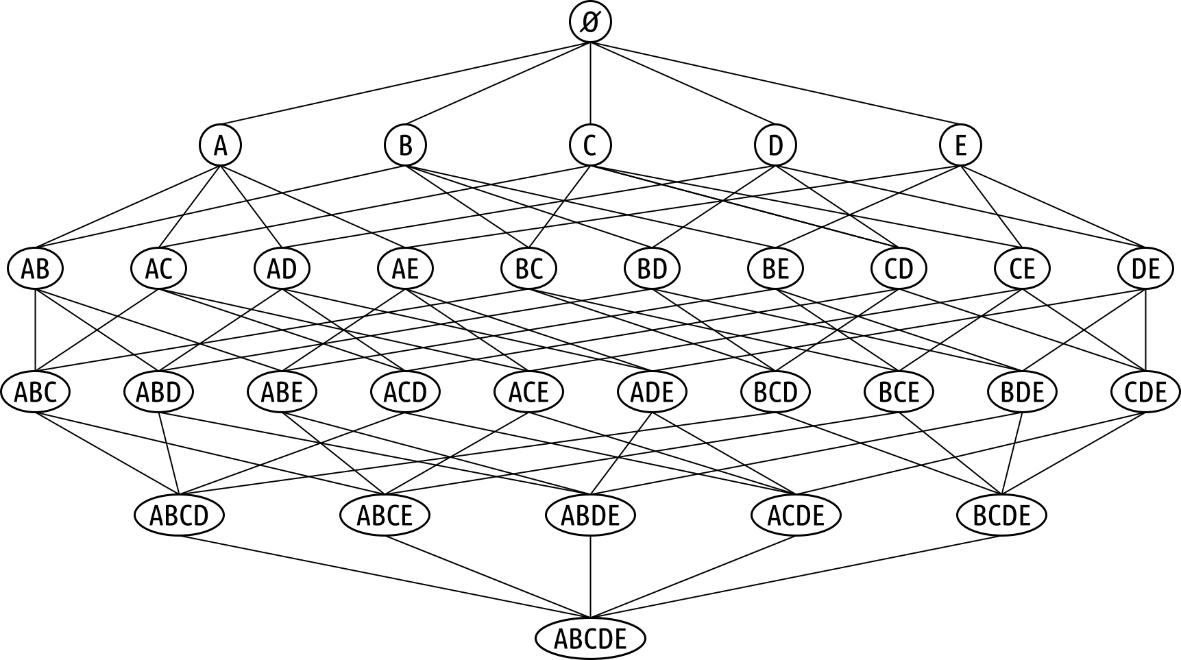
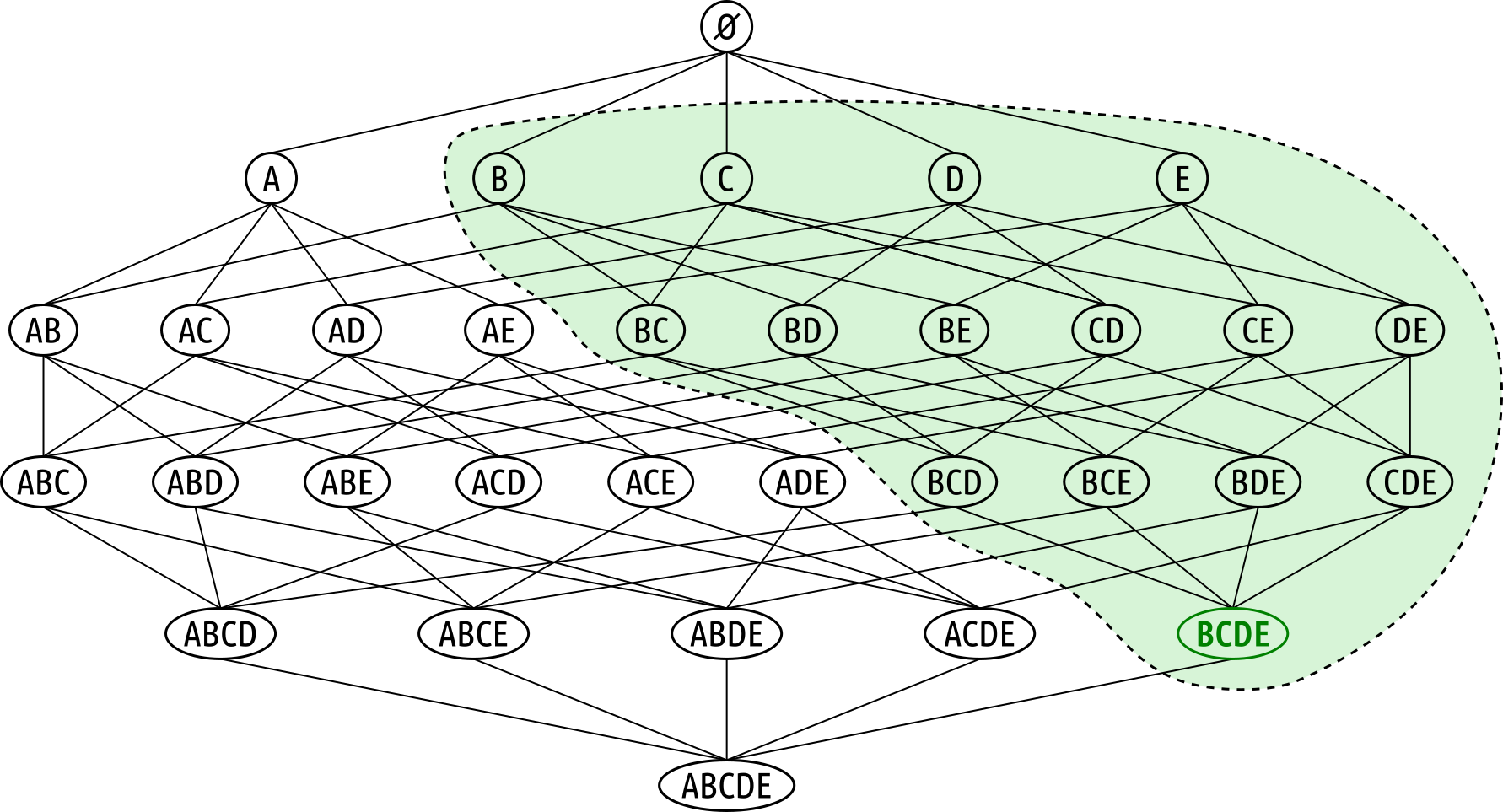
There are now two ways to utilize the anti-monotonicity property of support. Firstly, if we would know that an itemset, say, $\{B,C,D,E\}$ as sufficient support, we would also know that all itemsets that are a subset of $\{B,C,D,E\}$ also have sufficient support; the itemset lattice in the figure below shows all these itemset in a green region — we exclude the empty set since it is not useful in practice.
In principle, an algorithm could start with large itemsets and check which one has sufficient support. In practice, however, when dealing with large(r) sets of unique items $I$, this is problematic. For example, let's assume we have $100$ unique items — still small for practical application. For one, it's not obvious where to start. Since it is arbitrarily unlikely that transactions contain many items, starting with $100$-itemsets, $99$-itemsets, $98$-itemsets, etc. would be very wasteful — the likelihood that those itemsets are fequent is practically $0$. But if we would start with, say, $10$-itemsets, we would need to check $\large\binom{100}{10}\normalsize = 1,73\cdot 10^{13}$ itemsets. This is computationally prohibitive.
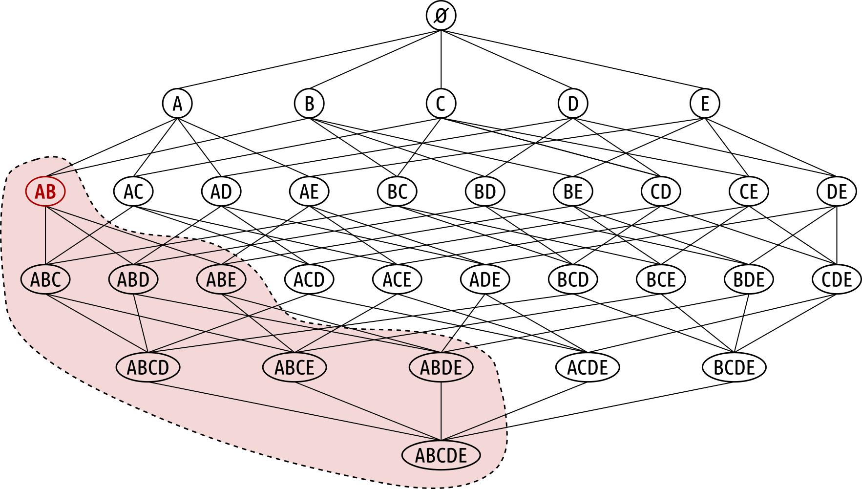
The alternative of utilizing the anti-monotonicity property of support is to identify small itemsets that do not have sufficient support since all supersets will also not have sufficient support. In the figure below showing the itemset lattice again, we assume that itemset $\{A, B\}$ has not sufficient support, i.e., $\{A, B\}$ is not a frequent itemset. This mean that all larger itemsets that have $\{A, B\}$ as a subset cannot be frequent itemsets as well, marked by the red region in the lattice.
This approach is arguably more straightforward since there is a meaningful way to start with checking $1$-itemsets and continue with checking larger itemsets ($2$-itemsets, $3$-itemsets, ...) — and always trying to minimize the itemsets we need to check using the anti-monotonicity property. This is therefore the underlying idea of the Apriori algorithm, which we describe in detail next.
Algorithm & Worked Example
The Apriori algorithm for generating all frequent itemsets is a bottom-up algorithm that starts with finding all frequent $1$-itemsets, all frequent $2$-itemsets, all frequent $3$-itemsets, and so on. The algorithm utilizes the anti-monotonicity property of support to only consider the $k$-itemsets that can be derived from the most recent frequent $(k\!-\!1)$-itemsets. To formalize the algorithm, let's introduce the following two notations.
- $L_k$: the set of candidate $k$-itemsets
- $F_k$: the set of frequent $k$-itemsets ($L_k\subseteq L_k$)
The algorithm is now an iterative process of finding all frequent $k$-itemsets for $k = 1, 2, 3, ..., |I|$ (at least in principle; in practice, the algorithm is likely to stop way before reaching $|I|$). To find the frequent $k$-itemsets in the $k$-th iteration, the algorithm performs the following $4$ core steps:
- GENERATE $L_k$ from $F_{k-1}$
- PRUNE $L_k$ using $F_{k-1}$
- COMPUTE support (count) for all itemsets in $L_k$
- FILTER $L_k$ itemset with sufficient support $\Rightarrow F_k$
- If $|F_k|=0$, stop; otherwise, go to 1.
The only special case here is that $L_1$ is the set of all candidate $1$-itemsets); using the notation above, we derive $L_1$ from $F_0$ which would be the set of frequent $0$-itemsets, which does not really exist (or we could say that this is the empty set).
Side note: Generally, the computationally most expensive step of this algorithm is computing the support (count) for each candidate item set in $L_k$. This is because computing the support (count) requires to actually go through the transaction database to count which transaction contain the candidate itemset. We therefore want to perform this step only for the candidate itemsets which we cannot exclude because of the anti-monotonicity property.
To see how the algorithm works, let's use it to find all frequent itemsets for our small Market Basket Analysis transaction database assuming $minsup = 0.2$ (which means a minimum support count of two since we have $5$ transactions). Recall that this database contains the following $5$ transactions:
| ID | Items |
|---|---|
| 1 | bread, yogurt |
| 2 | bread, cereal, eggs, milk |
| 3 | cereal, cheese, milk, yogurt |
| 4 | bread, cereal, milk, yogurt |
| 5 | bread, cheese, milk, yogurt |
Being a bottom-up algorithm, it starts with the smallest itemsets, i.e., the $1$-itemsets. Since we do not have any prior information at this point all $1$-itemsets are candidate itemsets. Therefore, we GENERATE $L_1$ simply the set of all unique items in $I$, represented by the following table; again, without prior knowledge, there is no possibility to further PRUNE $L_1$.
| Itemset |
|---|
| {bread} |
| {cereal} |
| {cheese} |
| {eggs} |
| {milk} |
| {yogurt} |
For all these $1$-itemsets, we need to COMPUTE the support count (SC) to see which of the itemsets is frequent or not. Given $minsup \geq 0.4$ and our $5$ transactions, we know that an itemset is frequent if it has an support count of at least $2$ — that is, the itemset occurs in at least $2$ transaction. We therefore have to scan the whole transaction database and count for each $1$-itemset its number of occurrences. The table below shows the results.
| Itemset | SC |
|---|---|
| {bread} | 4 |
| {cereal} | 3 |
| {cheese} | 2 |
| {eggs} | 1 |
| {milk} | 4 |
| {yogurt} | 4 |
The table above also indicates the FILTER step, where we remove all itemsets with insufficient support (here: $\{\text{eggs}\}$). This gives us $F_1$ the set of frequent $1$-itemsets and concludes our first iteration of the algorithm:
| Itemset |
|---|
| {bread} |
| {cereal} |
| {cheese} |
| {milk} |
| {yogurt} |
Since $F_1$ is not empty, we continue and GENERATE $L_2$ based on $F_1$. Most intuitively, since the $1$-itemset $\{\text{eggs}\}$ is not frequent, we can ignore all $2$-itemsets that have $\{\text{eggs}\}$. In other words, we generate $L_2$ as the set of all possible $2$-itemset we can form using the frequent $1$-itemsets — later, we discuss in more detail how we generate $L_k$ from $F_{k-1}$. Again, there is no further reason to PRUNE $L_2$ since we already ignored the $1$-itemsets that were now frequent.
| Itemset |
|---|
| {bread, cereal} |
| {bread, cheese} |
| {bread, milk} |
| {bread, yogurt} |
| {cereal, cheese} |
| {cereal, milk} |
| {cereal, yogurt} |
| {cheese, milk} |
| {cheese, yogurt} |
| {milk, yogurt} |
Fall these $2$-itemsets in $L_2$, we have to COMPUTE their support count (SC) by scanning the whole transaction database. The table below shows the counts for each itemsets and indicates the FILTER step by highlighting all the itemsets (here: $\{\text{bread, cheese}\}$ and $\{\text{cereal, cheese}\}$) with insufficient support.
| Itemset | SC |
|---|---|
| {bread, cereal} | 2 |
| {bread, cheese} | 1 |
| {bread, milk} | 3 |
| {bread, yogurt} | 3 |
| {cereal, cheese} | 1 |
| {cereal, milk} | 3 |
| {cereal, yogurt} | 2 |
| {cheese, milk} | 2 |
| {cheese, yogurt} | 2 |
| {milk, yogurt} | 3 |
After keeping only the itemsets with sufficient support, we get the set of frequent $2$-itemsets $F_2$:
| Itemset |
|---|
| {bread, cereal} |
| {bread, milk} |
| {bread, yogurt} |
| {cereal, milk} |
| {cereal, yogurt} |
| {cheese, milk} |
| {cheese, yogurt} |
| {milk, yogurt} |
$F_2$ is not empty, so we need to GENERATE $L_3$. We initialize $L_3$ by generating all possible $3$-itemsets we can form using items we find in $F_2$; note that $F_2$ still contains all items except for $\{\text{eggs}\}$. This gives us $\large\binom{10}{3}\normalsize = 10$ initial candadate $3$-itemsets. However, we can PRUNE this set by removing all $3$-itemsets we know cannot be frequent by utilizing the anti-monotonicity property of support. For example, consider the itemset $\{\text{bread, cheese, milk}\}$. This itemset contains the following three $2$-itemsets
- $\{\text{bread, cheese}\} \not\in F_2$
- $\{\text{bread, milk}\} \in F_2$
- $\{\text{cheese, milk}\} \in F_2$
Since at least one of these $2$-itemsets is not frequent (i.e., $\{\text{bread, cheese}\} \not\in F_2$), we know that $\{\text{bread, cheese, milk}\}$ cannot be frequent as well and can be removed from $L_2$; we do not have to compute the support count for this $3$-itemset. Based on this same logic we can remove all $3$-itemsets as indicated by the table below.
| Itemset |
|---|
| {bread, cereal, cheese} |
| {bread, cereal, milk} |
| {bread, cereal, yogurt} |
| {bread, cheese, milk} |
| {bread, cheese, yogurt} |
| {bread, milk, yogurt} |
| {cereal, cheese, milk} |
| {cereal, cheese, yogurt} |
| {cereal, milk, yogurt} |
| {cheese, milk, yogurt} |
After pruning, we need to COMPUTE the support count (SC) for the remaining $3$-itemset and FILTER $L_3$ by removing all itemsets that are not frequent, i.e., have insufficient support.
| Itemset | SC |
|---|---|
| {bread, cereal, milk} | 2 |
| {bread, cereal, yogurt} | 1 |
| {bread, milk, yogurt} | 2 |
| {cereal, milk, yogurt} | 2 |
| {cheese, milk, yogurt} | 2 |
This gives us the set of frequent $3$-itemsets $F_3$.
| Itemset |
|---|
| {bread, cereal, milk} |
| {bread, milk, yogurt} |
| {cereal, milk, yogurt} |
| {cheese, milk, yogurt} |
$F_3$ is not empty and we need to continue and GENERATE L_4. Intuitively, since $F_3$ still contains $5$ unique items, there are $\large\binom{10}{4}\normalsize = 5$ possible $4$-itemsets. However, we can be smarter about this by using $F_3$. Most importantly, we do not have to generate the $4$-itemset $\{\text{bread, cereal, cheese, yogurt}\}$ since $F_3$ does not contain the $3$-itemset $\{\text{bread, cereal, cheese}\}$ — again, we discuss smart ways to get from $F_{k-1}$ to $L_k$ later in more details.
This leaves us with four $4$-itemsets we can try to PRUNE further. In fact, all four $4$-itemsets can be pruned since all of them contain at least one $3$-itemset that is not frequent. To give and example, consider the $4$-itemset $\{\text{bread, cheese, milk, yogurt}\}$, which contains the following four $3$-itemsets:
- $\{\text{bread, cheese, milk}\} \not\in F_2$
- $\{\text{bread, cheese, yogurt}\} \not\in F_2$
- $\{\text{bread, milk, yogurt}\} \in F_2$
- $\{\text{cheese, milk, yogurt}\} \in F_2$
With at least one $3$-itemset not being frequent, itemset $\{\text{bread, cheese, milk, yogurt}\}$ cannot be frequent as well. This holds true for all initial $4$-itemsets in $L_4$, giving us:
| Itemset |
|---|
| {bread, cereal, cheese, milk} |
| {bread, cereal, milk, yogurt} |
| {bread, cheese, milk, yogurt} |
| {cereal, cheese, milk, yogurt} |
Of course, since $L_4$ is already the empty set, $F_4$ is also empty, without the need to compute any support counts.
| Itemset |
|---|
In other words, there are no frequent $4$-itemsets in our small transaction database, which naturally also means that there are no larger itemsets that are frequent. The algorithm therefore stops and returns the set of all frequent itemsets $F_1 \cup F_2 \cup F_3$ as its result.
On a conceptual level, the Apriori algorithm to compute all frequent itemsets is arguably rather straightforward. Of course, we skipped important implementation details. For example, we did not address how to efficiently COMPUTE the support counts by scanning the transaction database. However, most modern programming languages have built-in support to check if a set (i.e., an itemset) is a subset of another set (i.e., a transaction) to check if a transaction contains an itemset. There are other optimization techniques to speed up the costly scanning of the transaction database, but these are implementation details beyond the scope of this notebook.
However, as briefly mentioned before, there are some relevant alternatives to systematically GENERATE and PRUNE $L_k$ based on the $F_{k-1}$. So let's discuss them in a bit more detail.
Getting $L_k$
Recall that $L_k$ is the set of candidate $k$-itemsets for which we need to COMPUTE their support counts — the generally most expensive step in practice. We therefore want to keep $L_k$ as small as possible by utilizing the anti-monotonicity property of support to only consider the $k$-itemsets we cannot say for sure are not frequent. The information we need for this is in the set of frequent $(k\!-\!1)$-itemsets $F_{k-1}$. There are two main approaches to accomplish this.
$F_{k-1}\times F_{1}$ Method
As the name suggests, $F_{k-1}\times F_{1}$ method generates $L_k$ by merging the frequent $(k\!-\!1)$-itemsets with the frequent $1$-itemsets to get the initial candidate $k$-itemsets. The two tables below show the example where we want tot use $F_2$ and $F_1$ to get $L_3$.
|
|
When forming the candidate $3$-itemsets, we naturally only consider the combination of frequent $2$-itemsets and frequent $1$-itemsets that indeed form a $3$-itemset. For example, if we merge $\{\text{bread, cereal}\}$ and $\{\text{bread}\}$ (the first itemsets in both tables), we get $\{\text{bread, cereal}\}$ again which is not a $3$-itemset; so we ignore it. After merging the itemsets of both tables, we get the following initial set of candidate $3$-itemsets:
| Itemset |
|---|
| {bread, cereal, cheese} |
| {bread, cereal, milk} |
| {bread, cereal, yogurt} |
| {bread, cheese, milk} |
| {bread, cheese, yogurt} |
| {bread, milk, yogurt} |
| {cereal, cheese, milk} |
| {cereal, cheese, yogurt} |
| {cereal, milk, yogurt} |
| {cheese, milk, yogurt} |
Of course, we already know that we can further PRUNE this set by removing each candidate $3$-itemset that cannot be frequent because any $2$-itemset it contains is not frequent, i.e., is not in $F_2$. For example, we can remove $\{\text{bread, cereal, cheese}\}$ because $\{\text{bread, cheese}\} \not\in F_2$. After pruning all itemsets, we get the final list of candidate $3$-itemsets — which is, of course, the same set we got in the worked example above:
| Itemset |
|---|
| {bread, cereal, milk} |
| {bread, cereal, yogurt} |
| {bread, milk, yogurt} |
| {cereal, milk, yogurt} |
| {cheese, milk, yogurt} |
$F_{k-1}\times F_{k-1}$ Method
This method only uses the last set of frequent itemsets $F_{k-1}$. To illustrate this method, let's again assume that the last set of frequent itemsets we got for our example transaction database is $F_2$; see below.
| Itemset |
|---|
| {bread, cereal} |
| {bread, milk} |
| {bread, yogurt} |
| {cereal, milk} |
| {cereal, yogurt} |
| {cheese, milk} |
| {cheese, yogurt} |
| {milk, yogurt} |
The method now generates the initial candidate $k$-itemsets by merging all possible pairs of frequent $(k\!-\!1)$-itemsets that overlap in $(k\!-\!1)$ itemsets — otherwise, the merged itemset will not be a $3$-itemset. For example, if we merge $\{\text{bread, cereal}\}$ and $\{\text{milk, yogurt}\}$, we get $\{\text{bread, cereal, milk, yogurt}\}$, which is not a $3$-itemset. We obviously also do not merge a frequent $(k\!-\!1)$-itemset with itself as this would only yield the same $(k\!-\!1)$-itemset. If we do this for our example database, we get:
| Itemset |
|---|
| {bread, cereal, milk} |
| {bread, cheese, milk} |
| {bread, cereal, yogurt} |
| {bread, cheese, yogurt} |
| {bread, milk, yogurt} |
| {cereal, cheese, milk} |
| {cereal, cheese, yogurt} |
| {cereal, milk, yogurt} |
| {cheese, milk, yogurt} |
Although not very obvious for this small example database, this initial set of candidate $3$-itemsets differs from the one generated by the $F_{k-1}\times F_{1}$ method; and this is generally the case. However, after again pruning all candidate itemsets using the anti-monotonicity property of support, we get the same final set $L_3$:
| Itemset |
|---|
| {bread, cereal, milk} |
| {bread, cereal, yogurt} |
| {bread, milk, yogurt} |
| {cereal, milk, yogurt} |
| {cheese, milk, yogurt} |
Although both the $F_{k-1} \times F_{1}$ and $F_{k-1} \times F_{k-1}$ methods ultimately generate the same set of candidate $k$-itemsets, they differ in how candidates are produced and the amount of computation required. The $F_{k-1} \times F_{1}$ approach extends each frequent $(k\!-\!1)$-itemset by adding one frequent 1-itemset at a time, while ensuring that the resulting itemsets remain lexicographically ordered to avoid duplicates. This method is conceptually simple and easy to implement, making it useful for explaining the candidate generation process. However, it considers many unnecessary extensions that are later discarded because they violate the ordering constraint or fail the Apriori pruning step, resulting in additional computational overhead.
In contrast, the $F_{k-1} \times F_{k-1}$ approach performs a self-join of the frequent ((k-1))-itemsets, combining only pairs that share a common prefix of length $(k\!-\!2)$. As a result, every generated candidate already satisfies the structural conditions required to be a valid $k$-itemset, substantially reducing the number of candidate combinations that must be examined. Although this method requires a slightly more sophisticated join operation, it is significantly more efficient in practice and is the candidate generation strategy employed in the original Apriori algorithm. Thus, while both methods produce identical candidate sets, the self-join approach achieves this with considerably less redundant computation.
Basic Implementation
To really show that the Apriori algorithm for finding frequent itemsets is rather straightforward — at least conceptually, ignoring any finer optimization efforts — let's actually implement it in Python. Recall that we already have basic methods that compute the support association rules and itemset. For the main algorithm, we need two additional auxiliary methods. The first one is unique_items() which simply extracts the set of unique items across a transaction database. Applied to our example database, we get:
unique_items(db)
{'bread', 'cereal', 'cheese', 'eggs', 'milk', 'yogurt'}
Of course, this is nothing else than $I = \{\text{bread}, \text{cereal}, \text{cheese}, \text{eggs}, \text{milk}, \text{yogurt}\}$. However, with respect to the Apriori algorithm, this is also the set of candidate $1$-itemsets $L_1$.
The second auxiliary method is merge_itemsets() which takes in two arbitrary itemsets and returns their union. We need this method later when generating the next set of candidate $k$-itemsets $L_k$ based on the set of frequent $(k\!-\!1)$-itemsets $F_{k-1}$. The code cell below shows an example for using this method to merge two $2$-itemsets.
merge_itemsets(('bread', 'milk'), ('bread', 'eggs'))
('bread', 'eggs', 'milk')
Note that merge_itemsets() itemset sorts the items in the union. This is not needed, and we do it only so that the results look consistent, making it easier to compare them with the results from the worked example above.
We already highlighted that one core task of the algorithm is to systematically GENERATE and PRUNE $L_k$ based on the $F_{k-1}$; and we saw that this can be done in different ways. The method generate_Lk() in the code cell below implements the $F_{k-1}\times F_{k-1}$ method as described above. This method performs the two main steps:
- GENERATE: Merge/join all possible pairs of $(k\!-\!1)$-itemsets, but ignore all resulting itemset that are not of size $k$
- PRUNE: Only keep the $k$-itemsets of all its subsets of size $(k\!-\!1)$ are frequent, i.e., are in $F_{k-1}$.
At the end, method sorts all remaining itemsets. Again, this is not needed (and requires additional computation), and we do it only to improve readability.
def generate_Lk(Fk_minus_one):
    # Determine the next k from the set F_{k-1}
    # The code just looks a bit odd since we cannot get an element from a set using indexing
    k = len(next(iter(Fk_minus_one))) + 1

    # Initialize as set as a fail safe to avoid any duplicates
    Lk = set()

    for itemset1 in Fk_minus_one:
        for itemset2 in Fk_minus_one:

            # GENERATE candidate by merg/joining pair of itemsets
            k_itemset = merge_itemsets(itemset1, itemset2)
            # Ignore itemsets that are no of size k
            if len(k_itemset) != k:
                continue

            # PRUNE candidate by check if an (k-1) subset is not in F_{k-1}
            valid = True
            for p in generate_itemsets(k_itemset, min_len=(k-1), max_len=(k-1)):
                if p not in Fk_minus_one:
                    valid = False
            # Only keep candidate itemset of all (k-1) subsets are frequent
            if valid == True:
                Lk.add(k_itemset)

    return sorted(Lk) # (sorting not needed!!!)
Let's test this method by computing $L_3$, which means we need to pass $F_{2}$ as input. You can check the worked example to confirm that the set of $2$-itemsets with pass to method generate_Lk() as input indeed represents $F_2$ for our small transaction database (and $minsup = 0.4$).
k_itemsets = generate_Lk({
    ('bread', 'cereal'), ('bread', 'milk'), ('bread', 'yogurt'), ('cereal', 'milk'),
    ('cereal', 'yogurt'), ('cheese', 'milk'), ('cheese', 'yogurt'), ('milk', 'yogurt')
})

for itemset in k_itemsets:
    print(itemset)
('bread', 'cereal', 'milk')
('bread', 'cereal', 'yogurt')
('bread', 'milk', 'yogurt')
('cereal', 'milk', 'yogurt')
('cheese', 'milk', 'yogurt')
Of course, the output should match $L_3$ from our worked example.
We now already have everything to implement the Apropri algorithm for frequent itemset generation; the method frequent_itemsets_apriori() in the code cell below implements this algorithm. At the beginning, we handle the special case of generating the first set $L_k$ (i.e., $L_1$) as the set of unique items in the transaction database; of course, we use the method unique_items() to accomplish this.
The main part of the method is the the loop iterating over the core steps we introduced before
COMPUTE: Given the current set $L_k$, we compute the support for each itemset in $L_k$ (note that we compute the support here but computed the support count in the worked example; of course, the support is just the support count divided by the number of transaction $N$, which is a constant).
FILTER: We now remove all candidate $k$-itemsets with insufficient support to get the set of frequent itemsets $F_{k}$. A simple improvement of the algorithm would be to combine the COMPUTE and FILTER to avoid materializing the complete list of candidate $k$-itemsets and then filter them. However, this implementation makes it easier to see the connections to the core steps of the algorithm as introduced above.
GENERATE and PRUNE: If $F_{k}$ is not empty, we use the method
generate_Lk()to generate the next set of candidate itemsets (incl. the pruning step) and continue with the next generation
The method uses two dictionaries to record the information about all frequent itemsets:
itemset: The keys of this dictionary are $k$, i.e., the sizes of existing frequent itemsets, and the values for each $k$ are all frequent $k$-itemsets. We use this format as it mimics the return values of the implementation provided by theefficient-apriorilibrary; see below.cache: The keys of this dictionary are the frequent itemsets, and the values are their respective support values. We use this dictionary to have quick access to the support of any frequent itemsets, which we will later use to compute the confidence of association rules derived from those frequent itemsets.
In other words, just out of convenience, we essentially store and return the information about frequent itemsets twice.
def frequent_itemsets_apriori(db, min_support=0.5):
    # Initialize dictonary for final set of rules (keys are size of itemsets k)
    itemsets, cache = defaultdict(list), defaultdict(int)

    # GENERATE L1 = first set of candidate 1-itemsets
    Lk = set([(s,) for s in unique_items(db) ])

    while True:

        # COMPUTE support counts for all candidate itemsets
        Lk_support = [ (itemset, support_itemset(db, itemset)) for itemset in Lk ]

        # FILTER itemsets with sufficient support => those are frequent! (sorting not needed!!!)
        Fk = sorted([ (itemset, support) for (itemset, support) in Lk_support if support >= min_support])

        for itemset, support in Fk:
            itemsets[len(itemset)].append((itemset, support))
            cache[itemset] = support

        # If there's no k-frequent itemset, we can and should stop
        if len(Fk) == 0:
            break

        # GENERATE and PRUNE next set of candadiate k-itemsets
        Lk = generate_Lk([ itemset for (itemset, support) in Fk ])

    return itemsets, cache
Let's apply method frequent_itemsets_apriori() to our example database with $minsup=0.4$ to implement the worked example — and therefore see the same results. Since the result is organized with respect to the size of the frequent itemsets, we can print the itemsets for each existing value of $k$; just run the code cell below.
frequent_itemsets, cache = frequent_itemsets_apriori(db, min_support=0.4)

for k, itemsets in frequent_itemsets.items():
    print(f"Frequent {k}-itemsets:")
    for itemset in itemsets:
        print(itemset)
    print()
Frequent 1-itemsets:
(('bread',), 0.8)
(('cereal',), 0.6)
(('cheese',), 0.4)
(('milk',), 0.8)
(('yogurt',), 0.8)

Frequent 2-itemsets:
(('bread', 'cereal'), 0.4)
(('bread', 'milk'), 0.6)
(('bread', 'yogurt'), 0.6)
(('cereal', 'milk'), 0.6)
(('cereal', 'yogurt'), 0.4)
(('cheese', 'milk'), 0.4)
(('cheese', 'yogurt'), 0.4)
(('milk', 'yogurt'), 0.6)

Frequent 3-itemsets:
(('bread', 'cereal', 'milk'), 0.4)
(('bread', 'milk', 'yogurt'), 0.4)
(('cereal', 'milk', 'yogurt'), 0.4)
(('cheese', 'milk', 'yogurt'), 0.4)
Apart from comparing the output with the "manual" results from the worked example, we can also compare them with the implementation of the Apriori algorithm provided by the efficient-apriori library. The apriori() method of the library finds all association rules for a given minimum support and minimum confidence, however, also explicitly returns all frequent itemsets. Since the output format of the frequent itemset if our implementation matches the one of the efficient-apriori implementation, we can basically reuse the code:
itemsets, rules = apriori(db, min_support=0.4, min_confidence=1.0)

for k, itemsets in frequent_itemsets.items():
    print(f"Frequent {k}-itemsets:")
    for itemset in itemsets:
        print(itemset)
    print()
Frequent 1-itemsets:
(('bread',), 0.8)
(('cereal',), 0.6)
(('cheese',), 0.4)
(('milk',), 0.8)
(('yogurt',), 0.8)

Frequent 2-itemsets:
(('bread', 'cereal'), 0.4)
(('bread', 'milk'), 0.6)
(('bread', 'yogurt'), 0.6)
(('cereal', 'milk'), 0.6)
(('cereal', 'yogurt'), 0.4)
(('cheese', 'milk'), 0.4)
(('cheese', 'yogurt'), 0.4)
(('milk', 'yogurt'), 0.6)

Frequent 3-itemsets:
(('bread', 'cereal', 'milk'), 0.4)
(('bread', 'milk', 'yogurt'), 0.4)
(('cereal', 'milk', 'yogurt'), 0.4)
(('cheese', 'milk', 'yogurt'), 0.4)
Keep in mind that the value of min_confidence for the apriori() method does not affect the set of frequent itemsets since this set only depends on $minsup$. Feel free to try different values for min_confidence in the code cell above; it will not change the results.
With frequent_itemsets_apriori() we have implemented the computationally most intensive part of the Apriori algorithm, mainly because the COMPUTE step — which we have to do in each iteration — requires a complete scan of the transaction database. Still, we still want to find interesting association rules, not just frequent itemsets, which further depend on the minimum confidence threshold $minconf$.
Association Rule Generation
Simple Approach
Recall that we performed the step of frequent itemset generation to reduce the number of association rules for which we need to compute their confidence. Since $\text{Support}(X \rightarrow Y) = \text{Support}(X \cup Y)$, if we have a frequent itemset, we can derive all possible rules as all possible binary splits of that itemset (with nonempty antecedent and consequent). For example, if ${\text{bread, milk, yogurt}} is a frequent itemset, we get the following association rules:
- $\{\text{bread, milk}\} \rightarrow \{\text{yogurt}\}$
- $\{\text{bread, yogurt}\} \rightarrow \{\text{milk}\}$
- $\{\text{milk, yogurt}\} \rightarrow \{\text{bread}\}$
- $\{\text{bread}\} \rightarrow \{\text{milk, yogurt}\}$
- $\{\text{milk}\} \rightarrow \{\text{bread, yogurt}\}$
- $\{\text{yogurt}\} \rightarrow \{\text{bread, milk}\}$
Once enumerated, we have to check each rule if it has sufficient confidence and therefore should belong to the final result set. However, recall that:
This means that we can compute the confidence of a rule based on the support of the union $X\cup Y$ and the support of the antecedent $X$. The convenient observation now is that we already computed both values during frequent itemset generation, as both $X\cup Y$ and $X$ must be frequent itemsets. In other words, computing the confidence of an association rule does not require any additional scan of the transaction database. This allows for a straightforward implementation of this step; see below.
Apriori Extension
The simple approach evaluates all possible association rules that can be derived from a frequent itemset. Although computing the confidences for these rules is generally not computationally expensive, we can utilize the (constraint) anti-monotonicity property of confidence here to reduce the number of rules to consider.
To illustrate this, let's assume a frequent itemset $\{A, B, C, D\}$. We can now create all possible association rules and, again, organize them into a lattice. In this lattice, nodes are association rules and edges represent containment relationships with respect to the antecedent and consequent (depending on the "direction"). For example, there is an edge between the rules $\{\text{B,C,D}\}\rightarrow \{\text{A}\}$ and $\{\text{C,D}\}\rightarrow \{\text{A,B}\}$ (on the left) because the consequent $\{\text{A}\}$ of the first rule is a subset of the consequent $\{\text{A,B}\}$ of the second rule.
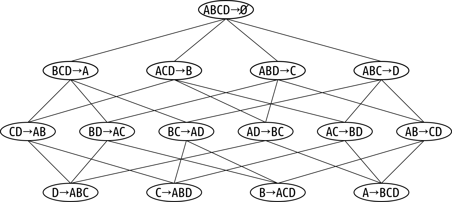
Recall that the anti-monotonicity property of confidence tells us that, if a rule $r$ does not have a sufficient confidence, all rules with a consequent that is a superset of the consequent of $r$. For example, if we would know that rule $\{\text{B,C,D}\}\rightarrow \{\text{A}\}$ has insufficient confidence, would also not that, say, rule $\{\text{B,D}\}\rightarrow \{\text{A,C}\}$ has insufficient confidence. The figure below shows the lattice, marking all the rules we do not need to check assuming the rule $\{\text{B,C,D}\}\rightarrow \{\text{A}\}$ has insufficient confidence.
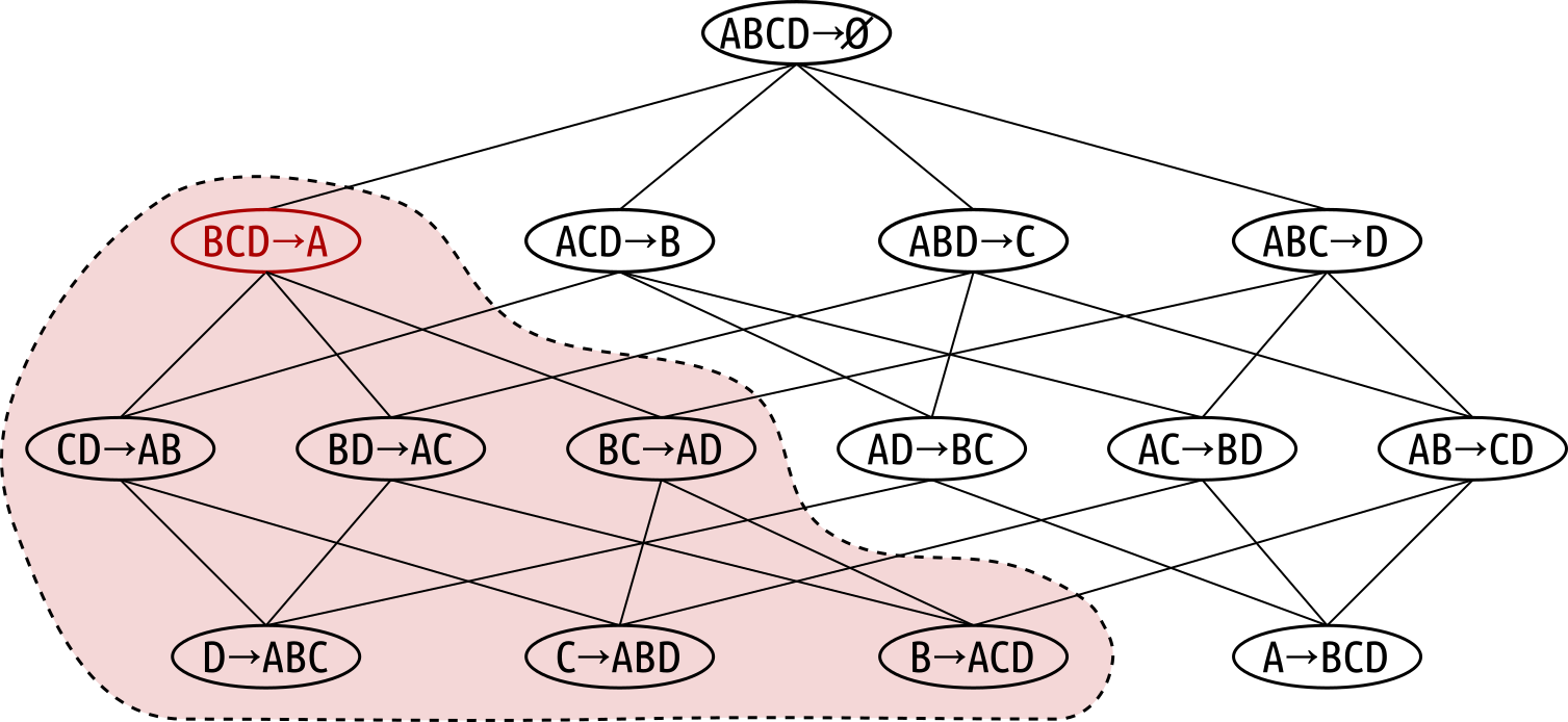
Side note: In the two figures above, the lattice shows the rule $\{\text{A,B,C,D}\}\rightarrow \emptyset$. This is only to give the lattice a "root". Of course, $\{\text{A,B,C,D}\}\rightarrow \emptyset$ is not a meaningful association rule and would not be considered as part of any algorithm.
Basic Implementation
Although implementing the Apriori extension of association rule generation is also quite straightforward — obviously very similar to the algorithm for frequent itemset generation — we keep things simple here and only implement the simple approach. While this means that we are likely compute the confidence of some rules unnecessarily, remember that we have all the required information (i.e., the support of frequent itemsets) to avoid any costly operations, particularly scanning the transaction database.
To implement the algorithm, we first need a simple auxiliary method that takes in an itemset to generate all possible rules as binary splits of the itemset. Since this is a generating task related to finding all subsets of a set, we do not focus too much on this method. But if you are interested you can check out the code for the method generate_rules(). Here is just a quick example that uses the method to generate all $6$ possible rules for a given $3$-itemset
for rule in generate_rules(('bread', 'cereal', 'milk')):
    X, Y = rule
    print(f"{X} --> {Y}")
('bread',) --> ('cereal', 'milk')
('cereal',) --> ('bread', 'milk')
('milk',) --> ('bread', 'cereal')
('bread', 'cereal') --> ('milk',)
('bread', 'milk') --> ('cereal',)
('cereal', 'milk') --> ('bread',)
In general, for any $k$-itemset, there are $2^k-2$ possible rules. This is because the number of all subsets of a set (i.e., its powerset) of size $k$ if $2^k$. However, we can ignore the empty set as well as the set itself (i.e., we only consider true subsets). Notice that the number of rules grows exponentially which does provide arguments for the Apriori extension for practical implementations. On the other hand, the size of even the largest frequent itemsets is typically not very large, particularly compared to the total number of unique items in the transaction database. And, again, we can compute the confidences of all rules using cached values.
The method myapriori() in the code cell below now implements the complete algorithm to find interesting association rules in a transaction database given minimum threshold values for support and confidence. Of course, the first step is to call frequent_itemsets_apriori() to generate all frequent itemset given the specified support. The nested loop then iterates over all frequent itemsets — recall that frequent_itemsets_apriori() returns a dictionary with the $k$ values being the keys, and the respective $k$-itemsets as the values. The, for each frequent itemset, we perform the following steps
Check if the itemset contains at least $2$ items; we cannot derive any rule from $1$-itemsets
Use the method
generate_rules()to generate all possible rules that can be derived from the current itemset; for each rule then do:- Split the rule into antecedent $X$ and consequent $Y$; recall that
ruleis always a $2$-tuple. This step is just to improve readability since we explicitly see where we need to work with $X$ and $Y$. - Get the support for $X$ and $Y$ from the cache, i.e., the result from the frequent itemset generation step; we only need support of $Y$ to compute the lift of the rule, see below, it is not require for the Apriori algorithm itself. Also, not that we already have the support of $X\cup Y$ from the 2nd
forloop! - Compute the confidence and the lift of the rule using the respective support values. We only compute the lift to mimic the output of the implementation of the
efficient-apriorilibrary. Since the lift does not have the anti-monotonicity property, its value does not affect the overall algorithm (i.e., the decision which rules are considered interesting). - If the rule has sufficient confidence, we add the rule together with its support, confidence, and lift to the final result set.
- Split the rule into antecedent $X$ and consequent $Y$; recall that
At the end, the myapriori() returns both frequent itemsets and interesting rules. Again, this is mainly to match the output of the efficient-apriori implementation.
def myapriori(db, min_support=0.5, min_confidence=0.5):
    # Initialize empty list of association rules
    rules = []

    # Find and loop over all frequent itemsets
    frequent_itemsets, cache = frequent_itemsets_apriori(db, min_support)

    # Iterate overall frequent itemsets
    for k, itemsets in frequent_itemsets.items():
        for itemset, support in itemsets:
            # We cannot generate rules from 1-itemset
            if len(itemset) == 1:
                continue
            # Find and loop over all association rules that can be generated from the itemset
            for rule in generate_rules(itemset):
                # Split rule into antecedent X and consequent Y
                X, Y = rule
                # Get support of antecendent X from cache
                support_X = cache[X]
                support_Y = cache[Y]
                # Compute confidence and lift
                confidence =  support / support_X
                lift = support / (support_X * support_Y)
                # Check if rules has a minimum confidence
                if confidence >= min_confidence:
                    rules.append((rule, {"supp": support, "conf": confidence, "lift": lift}))

    # Return final list of association rules
    return frequent_itemsets, rules
We can now finally find all the interesting rules for our small transaction database. In the code cell below, by default, we set $minsup=0.4$ and $minconf=1.0$ to match the previous "manual" examples. However, you are encouraged to play with both values to see how it affects the results.
itemsets, rules = myapriori(db, min_support=0.4, min_confidence=1.0)

for rule, measures in rules:
    X, Y = rule
    print(f"{X} -> {Y} ({measures})")
('cereal',) -> ('milk',) ({'supp': 0.6, 'conf': 1.0, 'lift': 1.25})
('cheese',) -> ('milk',) ({'supp': 0.4, 'conf': 1.0, 'lift': 1.2499999999999998})
('cheese',) -> ('yogurt',) ({'supp': 0.4, 'conf': 1.0, 'lift': 1.2499999999999998})
('bread', 'cereal') -> ('milk',) ({'supp': 0.4, 'conf': 1.0, 'lift': 1.2499999999999998})
('cereal', 'yogurt') -> ('milk',) ({'supp': 0.4, 'conf': 1.0, 'lift': 1.2499999999999998})
('cheese',) -> ('milk', 'yogurt') ({'supp': 0.4, 'conf': 1.0, 'lift': 1.6666666666666667})
('cheese', 'milk') -> ('yogurt',) ({'supp': 0.4, 'conf': 1.0, 'lift': 1.2499999999999998})
('cheese', 'yogurt') -> ('milk',) ({'supp': 0.4, 'conf': 1.0, 'lift': 1.2499999999999998})
Just for the sake of completeness, we can also compare the output with the one provided by the implementation of the Aprior algorithm provided by the efficient-apriori algorithm; see the code cell below. Naturally, to ensure matching results, we need to use the same values for $minsup$ and $minconf$. Note that this implementation also computes and outputs the conviction of each rule. However, we did not cover this measure in detail, so we omitted it in our implementations.
itemsets, rules = apriori(db, min_support=0.4, min_confidence=1.0)

for rule in rules:
    print(rule)
{cereal} -> {milk} (conf: 1.000, supp: 0.600, lift: 1.250, conv: 200000000.000)
{cheese} -> {milk} (conf: 1.000, supp: 0.400, lift: 1.250, conv: 200000000.000)
{cheese} -> {yogurt} (conf: 1.000, supp: 0.400, lift: 1.250, conv: 200000000.000)
{bread, cereal} -> {milk} (conf: 1.000, supp: 0.400, lift: 1.250, conv: 200000000.000)
{cereal, yogurt} -> {milk} (conf: 1.000, supp: 0.400, lift: 1.250, conv: 200000000.000)
{cheese, yogurt} -> {milk} (conf: 1.000, supp: 0.400, lift: 1.250, conv: 200000000.000)
{cheese, milk} -> {yogurt} (conf: 1.000, supp: 0.400, lift: 1.250, conv: 200000000.000)
{cheese} -> {milk, yogurt} (conf: 1.000, supp: 0.400, lift: 1.667, conv: 400000000.000)
Apart from the additional conviction values, the order of the rules, as well as the exact formatting of the output, both algorithms return the same set of interesting rules. That being said, the efficient-apriori implementation is better optimized and more flexible and should be preferred when working with large, real-world transaction databases — for our small example database, performance does not matter. The focus of our implementation was on clarity and understanding for educational purposes.
Limitations & Extensions
As we already briefly mentioned at the beginning, the basic Apriori algorithm as covered in this notebook makes a serious of simplifying assumption, mainly (using a Market Basket Analysis use case as an example):
- The algorithm only consider the presence or absence of items in a transaction but not any potentially relevant attributes such as quantity (e.g., $10$ vs. $100$ eggs) or price (e.g., cheap vs expensive items)
- Transactions are sets of items with no order. However, in online settings, it is very easy and can be very useful to track in which order items have been placed into the cart.
- Transactions are considered independent without consideration that multiple transactions may belong to the same customer
- The algorithm cannot handle incremental updates; by default, any change to the transaction based requires to run the algorithm again from scratch.
- The algorithm considers the database as a set of transactions without any additional attributes such as time to capture, e.g., seasonal patterns. However, this can partially be addressed by first filtering the transaction before passing a subset to the algorithm
While these assumptions greatly simplify the mining process and enable the efficient exploitation of the anti-monotonicity property of support, they are often too restrictive for real-world applications. Consequently, numerous extensions have been developed to incorporate additional information, such as item quantities, item utilities (e.g., profit or value), temporal and sequential information, product hierarchies, user characteristics, and continuously evolving or distributed datasets.
Despite these extensions, the fundamental idea underlying Apriori remains highly influential. Many Apriori variants, as well as entirely new frequent pattern mining algorithms, continue to exploit anti-monotonicity or closely related pruning principles to reduce the combinatorial search space efficiently. Consequently, the Apriori algorithm studied in this notebook should not be viewed merely as a single algorithm, but rather as the conceptual foundation of an entire family of algorithms for frequent pattern and association rule mining. Understanding its underlying principles therefore provides the basis for understanding many of the more advanced methods used in modern data mining.
Summary
This notebook introduced the Apriori algorithm for Association Rule Mining (ARM) using a simple running example to illustrate its key ideas. It began by introducing the fundamental measures of support and confidence, which quantify how frequently itemsets occur and how reliably one itemset implies another. A central observation was the anti-monotonicity property of support: if an itemset is infrequent, then all of its supersets must also be infrequent. This property forms the basis of Apriori's pruning strategy and makes efficient mining of large transaction databases possible.
Building on these concepts, the notebook motivated the decomposition of association rule mining into two separate tasks: frequent itemset generation and association rule generation. The first step identifies all itemsets whose support exceeds a user-defined minimum threshold, while the second derives association rules from these frequent itemsets that satisfy a minimum confidence threshold. Particular emphasis was placed on frequent itemset generation, as it constitutes the computationally most expensive part of the overall mining process and therefore determines the algorithm's efficiency.
The notebook then presented the Apriori algorithm in detail. It explained the level-wise generation of candidate $k$-itemsets from frequent $(k\!-\!1)$-itemsets, the pruning of candidates using the Apriori property, and the repeated support counting required to identify frequent itemsets. Subsequently, the generation of association rules from the discovered frequent itemsets was discussed, including the computation of confidence and the pruning of rules that do not satisfy the confidence threshold. Finally, all components were brought together in a complete from-scratch implementation of the Apriori algorithm, demonstrating how the theoretical concepts translate into executable code.
Although more advanced algorithms, such as FP-Growth and ECLAT, often outperform Apriori on large datasets, Apriori remains one of the most influential algorithms in data mining. Its simple yet powerful use of anti-monotonicity provides valuable insight into how combinatorial search problems can be solved efficiently through systematic pruning. Moreover, many modern frequent pattern mining algorithms build upon the same fundamental principles introduced by Apriori. For this reason, understanding the Apriori algorithm is essential for developing a solid foundation in association rule mining and data mining more broadly.