Disclaimer: This Jupyter Notebook contains content generated with the assistance of AI. While every effort has been made to review and validate the outputs, users should independently verify critical information before relying on it. The SELENE notebook repository is constantly evolving. We recommend downloading or pulling the latest version of this notebook from Github.
Artificial Neural Networks (Basic Architecture)
Artificial Neural Networks (ANNs) are a key technology in Artificial Intelligence (AI) inspired by the way the human brain works. Just like the brain uses neurons to process information, ANNs use artificial "neurons" to analyze and solve problems. They are a powerful tool for finding patterns in data, making predictions, and learning from experience, much like humans do. ANNs are at the heart of many AI applications we use every day. For example, they power facial recognition systems, language translation tools, voice assistants like Siri or Alexa, and even recommendation systems on platforms like Netflix and Spotify. Their ability to process large amounts of data quickly and identify complex patterns makes them crucial in areas like healthcare, finance, and robotics.
Learning about ANNs is important because they are driving much of the progress in modern AI. Whether you're a student, researcher, or professional, understanding how ANNs work can help you develop innovative solutions to real-world problems. They enable computers to perform tasks that were once thought to require human intelligence, such as recognizing images, predicting outcomes, or even creating original content. ANNs are also a foundation for other advanced AI methods, such as deep learning. By learning how ANNs function, you gain the skills needed to explore these cutting-edge areas. As AI continues to shape industries and improve lives, having knowledge of ANNs gives you the ability to contribute to this exciting field and stay ahead in a rapidly changing world.
In addition, understanding ANNs helps you think critically about their applications and limitations. While they are powerful, ANNs are not perfect and require careful design, training, and evaluation. By learning about them, you can better address challenges like bias in AI systems and make sure the technology is used responsibly and ethically. Overall, Artificial Neural Networks are a cornerstone of AI. Studying them opens the door to new opportunities in technology, research, and innovation. Whether you're curious about AI or looking to build a career in the field, ANNs are a great place to start!
Setting up the Notebook
Make Required Imports
This notebook requires the import of different Python packages but also additional Python modules that are part of the repository. If a package is missing, use your preferred package manager (e.g., conda or pip) to install it. If the code cell below runs with any errors, all required packages and modules have successfully been imported.
import numpy as np
The Artificial Neuron
An artificial neuron is a basic building block of a neural network, designed to mimic the way real neurons in the human brain work. Its primary purpose is to take in information, process it, and decide whether to pass it on to other neurons. In simple terms, it’s like a decision-maker that determines the importance of input data and sends relevant signals forward.
Each artificial neuron takes in inputs, like numbers or features from data, and multiplies them by weights that represent how important each input is. Then, it adds up these weighted inputs and passes the result through an activation function. This function decides whether the neuron "fires" or stays inactive, shaping the output in a way that helps the network learn patterns in data. By adjusting the weights during training, the neuron learns to focus on what matters most in solving a problem, like recognizing an image or predicting an outcome.
When many neurons are connected together in layers, they form a neural network capable of learning complex patterns and relationships. The artificial neuron's ability to filter and transform information is what makes these networks powerful tools for solving a wide range of problems, from language translation to medical diagnosis.
Inspiration: Biological Neuron
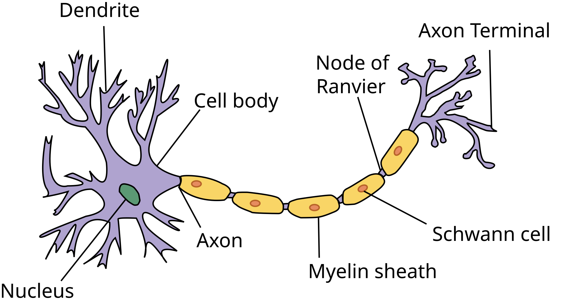
Source: "Anatomy and Physiology" by the US National Cancer Institute's Surveillance, Epidemiology and End Results (SEER) Program (Wiki Commons)
The main components of a biological neuron are:
Dendrite: A dendrite is a part of a neuron that looks like a branching tree. Its main job is to receive signals from other neurons and send them to the cell body of the neuron. These signals help the neuron decide whether to send its own message to other neurons. Dendrites have many branches, allowing them to connect with thousands of other neurons. They process the signals they receive, which can either excite or calm the neuron. This process is essential for how the brain and nervous system communicate and process information.
Cell body: The cell body, or soma, of a neuron is the central part of the cell that contains the nucleus. Its main purpose is to support the neuron's overall function by maintaining cell health and processing incoming signals. The cell body produces energy, proteins, and other materials needed for the neuron's activity. It also integrates the electrical signals received from the dendrites. If these signals reach a certain threshold, the cell body generates an action potential, which is then sent down the axon to communicate with other neurons or tissues.
Nucleus: The nucleus of a biological neuron is the control center of the cell, located within the cell body. Its main purpose is to regulate the neuron's activities, such as growth, repair, and the production of proteins necessary for communication and function. The nucleus contains the neuron's DNA, which holds the instructions for making proteins and other molecules.
Axon: The axon is a long, slender part of a neuron that transmits electrical signals, called action potentials, away from the cell body to other neurons, muscles, or glands. Its main purpose is to carry messages over long distances within the nervous system.
Axon terminal: The axon terminal, also called the synaptic terminal, is the endpoint of a neuron's axon. Its main purpose is to transmit signals to other neurons, muscles, or glands. It does this by releasing chemical messengers called neurotransmitters into the synapse, the small gap between neurons or other target cells.
Myelin sheath, Schwann cells, and nodes of Ranvier: The myelin sheath, Schwann cells, and nodes of Ranvier work together to ensure fast and efficient signal transmission along a neuron's axon. The myelin sheath is a fatty, insulating layer that surrounds the axon and speeds up electrical signal transmission by preventing signal loss and allowing it to travel more efficiently. Schwann cells produce and maintain the myelin sheath and assist in repairing damaged axons by promoting regrowth and regeneration after injury. Nodes of Ranvier are small gaps between segments of the myelin sheath along the axon. They play a key role in a process called saltatory conduction, where the electrical signal jumps from one node to the next. This dramatically increases the speed of signal transmission compared to an unmyelinated axon.
Biological Neuron vs. Logistic Regression
In a very simplified manner, we can describe the inner workings of a biological neuron as follows:
- A biological neuron receives input signals from other neurons through its dendrites. These inputs are combined in the cell body, where the neuron decides whether to "fire" or send an output signal. This process depends on the total input and a threshold. If the input exceeds the threshold, the neuron sends an output through its axon to the next neuron.
Now, let's consider equally simplified description of a Logistic Regression model:
- A Logistic Regression takes multiple input features, combines them using weights (similar to synaptic strengths in a neuron), and applies a mathematical transformation to decide the output. The combined inputs are passed through a sigmoid function, which produces a probability between 0 and 1. If the probability crosses a certain threshold, the output is classified into one category; otherwise, it falls into another.
In short, Logistic Regression can be considered a mathematical model of a biological neuron with several key parallels:
- Input Signals: In a biological neuron, these are electrical signals; in logistic regression, they are numerical feature values.
- Weights: Biological neurons use synaptic strengths, while logistic regression uses weights for input features.
- Combination of Inputs: Both systems sum their inputs before processing them further.
- Activation Function: Biological neurons use a thresholding mechanism; logistic regression uses the sigmoid function for probabilistic output.
Given these similarities, an artificial neuron is in essence nothing else than a Logistic Regression model; although, in the content of ANNs, the Logistic Regression model is often slightly modified, e.g., by using other activation functions beyond the Sigmoid function.
Of course, a biological neuron is much more complex than an artificial neuron because of its detailed structure and dynamic abilities. A biological neuron has parts like dendrites, the cell body, and axon, each with specific roles in receiving and sending signals. It also uses chemical signals (neurotransmitters) to communicate with other neurons. Biological neurons can adapt over time, change the strength of their connections, and learn from experience, making them highly flexible. On the other hand, artificial neurons are simpler mathematical models used in AI. They take inputs, process them, and produce an output based on a set of weights and an activation function. While artificial neurons can "learn" through training, their learning process is much more rigid and not as flexible as biological neurons. Biological neurons can also communicate in more complex ways and use less energy, making them far more efficient and robust compared to artificial neurons.
Assuming you are familiar with Logistic Regression, recall that a Logistic Regression model mapping in input $x$ to an output $y$ is defined as
where $\sigma$ is the Sigmoid function, $\mathbf{w}^T = [w_0, w_1, w_2, \dots, w_d]$ is the vector of weights (or parameters), and $\mathbf{x}^T = [x_1, x_2, \dots, x_d]$ is the vector of features. The image below shows a graphical representation of this computation which underpins Logistic Regression.
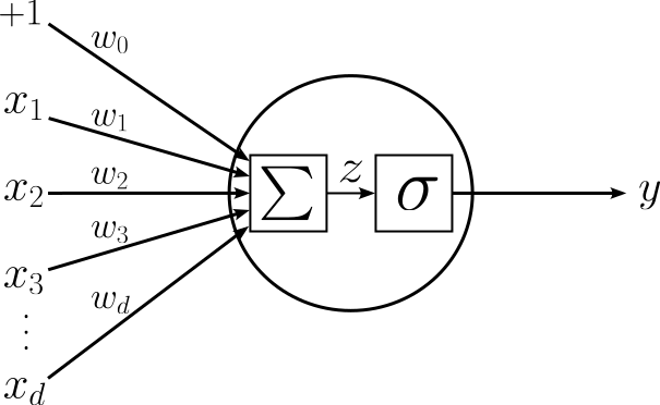
Here, $\sum$ represents the weighted sum of the input features:
with $x_0 = 1$ being the artificial feature to incorporate the bias weight $w_0$. As already mentioned, an artificial neuron may not exactly implement a Logistic Regression model. Particularly, an artificial neuron may feature an activation function that is not the Sigmoid function. Recall that Logistic Regression uses the Sigmoid function to ensure that the output $y \in [0, 1]$ and thus can be interpreted as a probability. As we will see later, the output of an artificial neuron that returns the final output of a neural network is generally not required to be interpreted as a probability. This allows for the application for a wide range of activation functions. Therefore, the more general graphical representation of an artificial neuron is shown below.
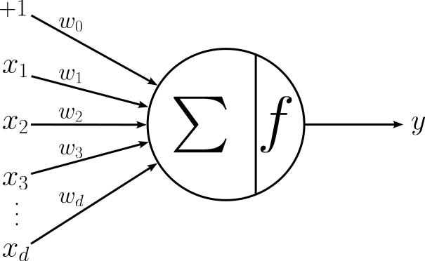
Here, $f$ is some activation function (Sigmoid or other). The important requirement is the $f$ is a nonlinear function. Again, we discuss this requirement later in full detail.
Limitations of a Single Artificial Neuron
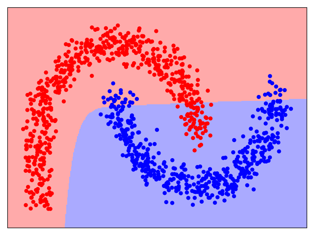
A single artificial neuron can be considered the smallest possible neural network. However, unsurprisingly, a single neuron — being essentially a Logistic Regression model — is a rather simple model. Logistic Regression, and hence a single neuron, is a binary classifier. This means that the decision boundary of a neuron that separates the classes is a straight line (in 2D), a plane (in 3D), or a hyperplane (in higher dimensions). However, for many real-world datasets, such simple decision boundaries are not suitable. To give an example consider the following figure. It shows the data distribution of a binary classification dataset (Class $Red$ and Class $Blue$), as well as the decision boundary a Logistic Regression model would learn.
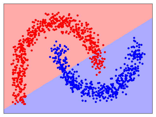
It is very easy to see that there is no way that the data points of this dataset can be meaningfully separated using a line as a decision boundary. While training a Logistic Regression model still finds the best line, the model will make a lot of errors over the training data — that is, all $Red$ data points in the $Blue$ area, and all $Blue$ data points in the $Red$ area. What we want is a model that allows for more intricate decision boundaries to better capture more complex data distributions. And this limitation of a single neuron brings us to the concept of neural networks as the systematic combinations of many neurons.
The Basic ANN Architecture
Most fundamentally, the basic architecture of an Artificial Neural Network (ANN) combines multiple artificial neurons into a network of neurons by
- Organizing multiple neurons into layers, and
- Stacking multiple layers together.
In the following, we look in more detail into both concepts how together the support, at least in principle, arbitrary complex decision boundaries.
Layers of Neurons
A (network) layer is a set of neurons that all receiving the same input. Organizing multiple neurons into a single layer the network to process and analyze multiple aspects of the input data simultaneously. Each neuron in a layer functions as a small "detector" applying its own set of weights and biases that focuses on specific patterns or features in the data. Another way to think about it is that each neuron produces its own decision boundary (as we will see later). This allows the layer as a whole to capture a wide variety of features or patterns in the data.
The figure below shows an example, where the same input — here represented by only two variables $x_1$ and $x_2$ — is fed into a layer containing $4$ neurons; we say that the layer has a size of $4$. Notice that we denote the output of a neuron with $a$ (for activation) since $y$ is generally reserved for the final output of a network (and we will see in a bit the output of a layer may not be the final output of a network).
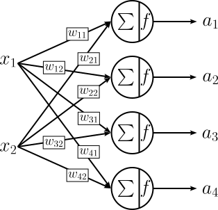
Since each neuron comes with its own set of weight, uniquely identifying a single weight becomes a bit more complex. A common convention for denoting a weight is $w_{ji}$ where $j$ is the $j$-th neuron in the layer and $i$ is the $i$-th input. Notice that the figure above is missing the bias value "$+1$" and the associated weights $w_{10}$, $w_{20}$, $w_{30}$, ..., $w_{d0}$. This is commonly done to simplify the visualization of ANNs, but remember that each neuron has its own bias term. Based on this, we can also calculate the number of weights for a layer with $d$ neurons and $k$ inputs as:
For example, in line with the figure above, if a layer has $d=d$ neurons each receiving the same $k=2$ inputs, the number of required weights is $2\cdot 4 + 4 = 12$.
Using this notation for the weights, we can now also express the output $a_j$ of the $j$-th neuron in the layer:
We use $b_{j}$ to denote the bias weight $w_{j0}$. The only reason for this is to adhere to common conventions in the neural network literature. The express the output of the complete layer (i.e., all individual outputs $a_1$, $a_2$, $a_3$, ..., $a_d$) as a single equation we combine all weights (incl. biases) and inputs into matrices and vectors:
where the weight matrix $\mathbf{W}$ is of size $d\times k$, input vector $\mathbf{x}$ is of size $k\times 1$, and bias vector $\mathbf{b}$ is of size $d\times 1$; more specifically:
The output vector $a$ is of size $d\times 1$. All matrix and vector elements are real numbers.
Stacking of Layers
Instead of treating the output of a neuron — or more commonly of a layer of neurons — as the final output of the model, we can use the output of one layer as the input for a subsequent layer. Using a sequence of layers offers significant advantages over single-layer architectures, particularly in its ability to model complex, non-linear relationships within data. Each layer enables the MLP to learn increasingly abstract representations of the input features, allowing it to capture patterns that would be impossible to represent with a single layer.
The figure below shows the basic stacking of two layers; again we omit the bias to ease presentation. In this example, the output of a layer containing 4 neurons serves as input of a subsequent layer containing 3 neurons. According to the definition of a layer, each of the 3 neurons in the second layer gets the same 4 inputs from the first layer.
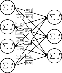
The total number of weights is again $kd + d$, just that now $k$ is the number of neurons in the first layer and $d$ is the number of the neurons in the second layer.
Of course, at least in principle, an ANN may have an arbitrary amount of layers. The last layer of an ANN is called the output layer. Any other layer — that is, a layer whose output serves as input for another layer — are called a hidden layer. All input features form the so-called input layer. As such, a basic ANN has $1$ input layer, $N$ hidden layers, and $1$ output layer.
Full Architecture
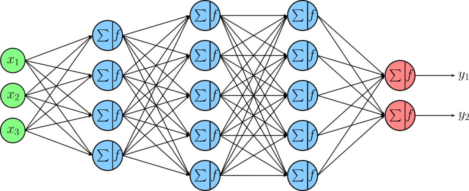
Combining the two core concepts of organizing neurons into layers and then connecting layers by using the output of one layer as the input for a next layer brings us the basic architecture of an Artificial Neural Network (ANN). The figure below shows an example network with
An input layer representing inputs described by three features $x_{1}$, $x_{2}$, and $x_{3}$.
Three hidden layers if sizes 4, 5, and 5.
An output layer containing two neurons to return the final output values $y_1$ and $y_2$ of the network.
As before, this figure does not show the bias weight for each neuron in the hidden layers and the output layer.
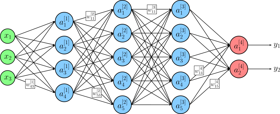
To properly describe an ANN and uniquely identify each individual weights and each individual output of a neuron, we have to further extend the mathematical notation. Most importantly, we need a way to address individual layers:
$\large L$: the total number of layers (containing neurons, this excluding the input layer). Our example network above has four layers, hence $L=4$.
$\large d^{[l]}$: the total number of neurons in layer $l$, with $1 \leq l \leq L$. For out example network, we have $d^{[1]}=4$, $d^{[2]}=5$, $d^{[3]}=5$, and $d^{[4]}=2$.
$\large w_{ji}^{[l]}$: the weight of the $j$-th neuron in the layer $l$ associated with the output of the $i$-th neuron or input of layer $(l-1)$.
$\large a_{i}^{[l]}$: the output of the $i$-th neuron in layer $l$.
Given these definitions we can revise the example network architecture as shown. Neurons are now labeled by their output $a$ (for activation); to avoid cluttering, the figure includes only some selected weights $w$.
The output of an ANN is calculated layer by layer, starting from the input layer, through all hidden layers, and finally the output layer. If we define $a_{i}^{[0]} = x_{i}$, we can define define the output of each neuron in the network as follows:
We can now define the output of $l$-th layer as:
where $\mathbf{a}^{[0]} = \mathbf{x}$; where weight matrix $\mathbf{W}^{[l]}$ is of size $d^{[l]}\times d^{[l-1]}$, input vector $\mathbf{a}^{[l]}$ is of size $d^{[l-1]}\times 1$, and bias vector $\mathbf{b}^{[l]}$ is of size $d^{[d]}\times 1$; more specifically:
The output $\mathbf{a^{[l]}}$ of a layer $l$ is calculated "in one go". Calculating $\mathbf{a^{[l]}}$ relies solely on matrix and vector operations which can be highly parallelized using GPUs (Graphical Processing Units) or TPUs (Tensor Processing Units). GPUs and TPUs are special types of hardware designed to handle many calculations at the same time, making them much faster than regular CPUs for certain tasks. GPUs were originally built for rendering graphics in video games, but their ability to perform lots of calculations in parallel makes them great for training neural networks. TPUs are even more specialized. They are designed specifically for machine learning tasks, especially for training and running deep neural networks. Unlike GPUs, which are general-purpose, TPUs are built to process the kinds of math (like matrix multiplications) that neural networks rely on. This makes TPUs faster and more efficient than GPUs for many machine learning tasks, especially at a large scale.
Using the notation for denoting the output of a layer, we can see that the output $\mathbf{\hat{y}}$ of a network is the output of the last layer, i.e., layer $L$. This means that $\mathbf{\hat{y}} = \mathbf{a}^{[L]}$, and using the equation above, we can calculate the output $\mathbf{\hat{y}}$ as:
As the output $\mathbf{a}^{[L]}$ of the last layer $L$, depends on the output $\mathbf{a}^{[L-1]}$ of the previous, i.e., second-to-last, layer $L-1$. Of course, now the output $\mathbf{a}^{[L-1]}$ depends on the output of $\mathbf{a}^{[L-2]}$. This recursive definition of the network output $\mathbf{y}$ continues until we reach the initial input $\mathbf{a}^{[0]} = \mathbf{x}$; more formally:
This equation illustrates the layer-wise computation of the network output, where the input $\mathbf{x}$ is transformed by each hidden layer and finally the output layer to yield $\mathbf{\hat{y}}$.
Layer-wise Calculation — Worked Example
Let's go through a complete example for the layer-wise calculation of the output of an ANN. To keep it simple — but also align it with a later discussion — we consider a very small network with only a single hidden layer of three neurons. An input $\mathbf{x}$ has only two features: $x_1$ and $x_2$. The output layer has only a single neuron. We consider a binary classification just like basic Linear Regression. Thus, the activation function of the output neuron is the Sigmoid function. Although not mandatory, we also assume the activation function of the hidden layer to be the Sigmoid function. In short, each neuron in the network indeed mimics a Logistic Regression model. The figure below visualizes our small ANN.
Again, we do not explicitly show the bias in the previous figure. However, for actually calculating the output of the networks from input, we do have to consider all biases.
Doing the Math
Based on our definitions above, we calculate the output of the first (and only) hidden layer using $\mathbf{a}^{[1]} = \sigma \left( \mathbf{W}^{[1]}\mathbf{x} + \mathbf{b}^{[1]} \right)$. Throughout this example, we assume some random input $\mathbf{x}$, random weight matrices $\mathbf{W}^{[l]}$, and random biases $\mathbf{b}^{[l]}$. We will be using the same value when we actually implement these calculations in Python. With this, we can calculate $\mathbf{a}^{[1]}$ as:
We already know that $\mathbf{a}^{[1]}$ is not the input for layer 2, which here is already our output layer that will give us $y$. Once again, assume some random entries for the weight matrices and biases, we can calculate $\mathbf{y} = \mathbf{a}^{[1]}$ as:
Notice that the output is a vector containing a single element. In principle the approach can be done for multiple inputs $\mathbf{x}$ in parallel. The only difference is that the input vector $\mathbf{x}$ becomes an input matrix $\mathbf{X}$, as well as all layer outputs $\mathbf{a}^{[l]}$ become a matrix where the number or columns reflect the number of input data samples.
As usual, when using the Sigmoid function as the activation function for a single output, we can interpret $y$ again as a probability. In other words, the probability that the example input vector $\mathbf{x}$ belongs to Class 1 is about $70%$.
Implementation with NumPy
Now that we have seen how the math for calculating the output of an ANN works using a concrete example, let's actually implement this calculation with Python. For this we use NumPy as this library is very convenient and highly optimized for matrix and vector operations — which is all we need to do. The implementation will use the same values for the input, weights, and biases, so you can directly match the math to the code.
The only custom method we first have to implement is the Sigmoid function. But again, using the power of NumPy, this can be done using a single line of code; however, having a dedicated method for implementing the Sigmoid function makes subsequent code easier to read. The code cell below contains the implementation of method sigmoid():
def sigmoid(z):
    return 1.0/(1.0 + np.exp(-z))
The next code simply randomly generates the input, weights, and biases. To ensure that all values match the ones we used in the math calculations above, we need to set the random seed here to 5. You are welcome to change the seed to get a different input, and different weights and biases to see how the outputs of the layers change. Of course, then those results will no longer match the example calculations done using math above.
# Set random seed to ensure that the values reflect the math equation above
np.random.seed(5)
# Create random input features
x = np.random.uniform(-1, 1, size=(2,1)).round(decimals=2)
# Create random weights and bias for hidden layer (l=1)
W1 = np.random.uniform(-1, 1, size=(3,2)).round(decimals=2)
b1 = np.random.uniform(-1, 1, size=(3,1)).round(decimals=2)
# Create random weights and bias for output layer (l=2)
W2 = np.random.uniform(-1, 1, size=(1,3)).round(decimals=2)
b2 = np.random.uniform(-1, 1, size=(1,1)).round(decimals=2)
We can now implement the calculation of the output $\mathbf{a}^{[1]}$ of the first and only hidden layer. Using the NumPy library, this again can be done using a single line of code. Appreciate how the line sigmoid(np.dot(W1, x) + b1) directly reflects out basic calculation $\mathbf{W}^{[1]}\mathbf{x}+\mathbf{b}^{[1]}$. The dot() method in NumPy is used to compute the dot product of two arrays. For 1D arrays, it performs the standard vector dot product, while for 2D arrays, it acts as matrix multiplication. While not required in this concrete example, it can also handle higher-dimensional arrays, where it sums the product of elements along specified axes, making it a versatile tool for Linear Algebra operations.
a1 = sigmoid(np.dot(W1, x) + b1)

print("Output of 1st layer a1:")
print(a1.round(decimals=2))
Output of 1st layer a1:
[[0.63]
 [0.39]
 [0.25]]
Notice that the shown result is rounded to ease the presentation. With $\mathbf{a}^{[1]}$ as the input for the next layer (i.e., the output layer), we can perform the exact same operations to calculate $\mathbf{a}^{[1]}$.
y = sigmoid(np.dot(W2, a1) + b2)

print("Output of 2nd layer a2 (final output y of the network):")
print(y.round(decimals=2))
Output of 2nd layer a2 (final output y of the network):
[[0.7]]
Intuitively, if our network would have more hidden layers, this process would simply continue layer by layer.
We can see that by using methods for matrix and vector operations, calculating the output of an ANN is very easy to implement. Of course, so far, we only assume some give weights and biases and did not actually train the network. However, this is beyond our scope here and will be covered in full detail in a separate notebook.
The Power of ANNs (Illustrated)
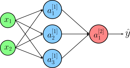
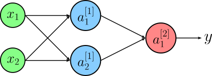
Now that we covered the fundamental architecture of an ANN, how does such a neural network go beyond the limitations of a single Logistic Regression model? To give a basic intuition for the capacity of an ANN, let's consider our initial binary classification dataset and see how different ANNs perform. In fact, we use the same simple ANN we used for the worked example above, containing only a single hidden layer. The number of inputs ($2$) and the number of output neurons ($1$) match the nature of the dataset and the binary classification tasks. Again, all neurons use the Sigmoid function for their activation.
The only parameter of the network architecture we vary is the number of neurons in the hidden layer. In the following, we consider $1$, $2$, and $3$ neurons for the hidden layer. Note that if the hidden layer contains only a single neuron, the network "collapses" to a simple Logistic Regression model, as the neuron in the output layer receives only one input. The output neuron has therefore no additional way to learn something "new" from combining multiple outputs. The images below show the three network architectures together with the decision boundaries they are able to learn.
 |
|
 |
 |
|
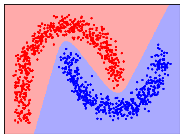 |
In very simple terms, we can see how each neuron in the hidden layer can model a different decision boundary, and the output neuron then combines them to the final decision boundary shown in the scatter plots above. More generally, the organization of neurons into layers and the combination of their outputs by subsequent layers allows the network to model nonlinear functions mapping the input to some output, which a Logistic Regression model is not capable of.
Just by looking at the examples, you might wonder if by simple adding more and more neurons to the hidden layer a network could model any non-linear functions. And this is indeed correct! The Universal Approximation Theorem states that a feedforward neural network with a single hidden layer containing a sufficient number of neurons can approximate any continuous function on a compact domain, provided it uses a non-linear activation function. This highlights the theoretical power of neural networks to model complex relationships between inputs and outputs. It provides the foundation for understanding why neural networks can be effective in tasks like image recognition, natural language processing, and other areas of machine learning. However, while the theorem demonstrates that a single hidden layer is sufficient in theory, there are practical reasons why neural networks often utilize multiple hidden layers:
Efficiency and Scalability: A single hidden layer network may require an impractically large number of neurons to approximate complex functions, leading to increased computational costs and difficulty in training. Deep networks, with multiple hidden layers, can represent complex functions more compactly by learning hierarchical features. Each layer captures increasingly abstract features (e.g., edges in the first layer, textures in the second, and objects in higher layers in image processing tasks), making the model both more efficient and interpretable.
Training and Generalization: Deep networks often generalize better to unseen data than wide, shallow networks. Multiple layers allow the network to decompose a task into simpler subtasks, with each layer specializing in different aspects of the data. This hierarchical learning reduces the risk of overfitting, especially when combined with regularization techniques like dropout or weight decay.
Optimization Challenges: While the theorem guarantees the existence of a solution for a single-layer network, it doesn’t address the difficulty of finding that solution through training. In practice, deep networks are often easier to train with modern optimization techniques like backpropagation and gradient descent, especially when paired with activation functions that mitigate issues like vanishing gradients.
In summary, while the Universal Approximation Theorem demonstrates the theoretical capability of single-layer networks, the practical advantages of efficiency, generalization, and trainability make multiple hidden layers the preferred choice in modern deep learning architectures.
Summary & What's Next?
In this notebook, we covered the basic architecture of Artificial Neural Network, how it can be seen as an "evolution" of Logistic Regression. The architecture consists of layers of interconnected neurons, on a high level mimicking the way biological neurons process information. An ANN typically has three types of layers: the input layer, which receives data; one or more hidden layers, where computations and transformations occur; and the output layer, which provides the final prediction.
Logistic regression can be seen as a simple neural network with no hidden layers, where a single output neuron uses the Sigmoid activation function to predict probabilities for binary classification. In this sense, logistic regression serves as the foundation for ANNs, and extending it with additional layers and neurons allows ANNs to handle more complex, non-linear relationships in data. Thus, ANNs generalize the principles of Logistic Regression, making them highly versatile for various machine learning tasks.
While we have seen how the output of an ANN is generated through layer-wise calculations using matrix and vector operations, we so far skipped the actual training of a network; which will walk about in a separate notebook. However, assuming you are familiar with training or fitting a Logistic Regression model, training an ANN involves the exact same principle steps. Appreciate that whether having a single neuron (i.e., Logistic Regression) or many neurons organized in many stacked layers, a neural network can always bees as as some function, commonly denoted as $\mathbf{\hat{y}} = h_{\mathbf{w}}(\mathbf{x})$ that maps some input $\mathbf{x}$ to some output $\mathbf{x}$ based in some internal parameters or weights $\mathbf{w}$. As such, the training of an ANN comes down to the same two steps as for Logistic Regression:
Definition of a suitable loss function $L(\hat{\mathbf{y}}, \mathbf{y})$ to quantify the difference between the predicted and the true class labels with respect to a current set of weights $\mathbf{w}$ to assess how well a network performs on a classification or predictions task.
Application of a suitable training strategy to systematically the best (or close to best) weight parameters $\mathbf{w}$ that minimize the loss function $L$.
In the case of Logistic Regression, the loss function of choice was the Cross-Entropy Loss, and we could use Gradient Descent to minimize that loss function. And in fact, for basic classification tasks, ANNs also rely on the Cross-Entropy Loss and Gradient Descent for their training. That being said, the function $h_{\mathbf{w}}(\mathbf{x})$ described by an ANN with many layers and neurons per layer is much more complex compared to $h_{\mathbf{w}}(\mathbf{x})$ for Logistic Regression:
With $y = h_{\mathbf{w}}(\mathbf{x})$ being more complex, the loss function $L(\hat{\mathbf{y}}, \mathbf{y})$ will naturally also be more complex. This makes the calculation of the gradient to train the network by iteratively updating the weights $\mathbf{w}$ much more challenging. Similar to the layer-wise calculation of the output of an ANN (see above), the calculation of the gradients is also done layer by layer via the process of backpropagation which starts at the output layer and calculates the gradient by going back through the network until the input layer.
The complexity of $L(\hat{\mathbf{y}}, \mathbf{y})$ also causes the loss function to be no longer convex like the Cross-Entropy Loss for Logistic Regression. This means that $L$ no longer has a single minimum, but can have many local minima and saddle points. This makes efficiently training large ANN much more challenging compared to much simpler models such as Logistic Regression.
Large ANNs may have a huge amount of trainable weights $\mathbf{w}$. This gives ANNs the capacity to learn very complex nonlinear functions. On the flips side, this increased model capacity also increases the risk of overfitting, i.e., the risk of the model learning the noise in the training data and therefore performing poorly on new unseen data. Training large ANNs therefore requires effective regularization techniques.
All the topics and techniques will be covered in detail in separate notebooks.