
Disclaimer: This Jupyter Notebook contains content generated with the assistance of AI. While every effort has been made to review and validate the outputs, users should independently verify critical information before relying on it. The SELENE notebook repository is constantly evolving. We recommend downloading or pulling the latest version of this notebook from Github.
KV Caching
Large Language Models (LLMs) have transformed artificial intelligence, but deploying them efficiently remains a major engineering challenge. During text generation — a process known as autoregressive decoding or inference — the model generates output one token (or word) at a time. To predict each new token, the model must process the entire sequence of previous tokens through its neural network layers. Because multi-head attention calculates how every token in a sequence interacts with every other token, computing these representations from scratch at every single generation step creates an immense computational bottleneck, rendering inference unacceptably slow and resource-intensive.
A closer look at the mathematics of self-attention reveals a massive redundancy: Autoregressive generation, combined with the way self-attention operates, also leads to repeated computation of the same intermediate results. At each step, the model must attend to tokens that were processed during earlier steps, even though their key and value representations have already been computed and will not change. Key-Value (KV) Caching exploits this observation by storing the key and value vectors from previous forward passes and reusing them during subsequent generation steps. The model only needs to compute the new key and value vectors for the newly generated token, rather than recomputing them for the entire sequence.
By eliminating redundant matrix multiplications, KV Caching dramatically accelerates generation speed and has become an absolute industry standard for efficient LLM inference. However, this performance boost comes with a distinct trade-off: memory overhead. While model weights occupy a fixed amount of VRAM, the KV Cache grows dynamically with every generated token, scaling linearly with batch size, context length, number of layers, and hidden dimensions. In modern long-context applications, the memory footprint of the KV cache can easily dwarf the memory required by the model weights themselves, leading to out-of-memory errors or limiting concurrent server throughput.
Understanding how KV Caching works — and how to manage its substantial memory footprint — is crucial for anyone building, optimizing, or deploying modern Transformer models. In this notebook, we provide a detailed look into why and how KV Caching works, showing the underlying math but also practical example use a from-scratch implementations of attention with and without the use KV Caching. We also discuss the memory overhead KV Caching introduces and briefly outline popular strategies to reduce the memory footprint.
Setting up the Notebook
Make Required Imports
This notebook requires the import of different Python packages but also additional Python modules that are part of the repository. If a package is missing, use your preferred package manager (e.g., conda or pip) to install it. If the code cell below runs with any errors, all required packages and modules have successfully been imported.
import numpy as np
import pandas as pd
import torch
import torch.nn as nn

from src.utils.plotting.math import *
Preliminaries
- This notebook assumes a basic understanding of the attention mechanism (including causal masking) and the Transformer architecture; however, the notebooks start with a brief recap about attention.
- All examples shown throughout the notebook use proper words as token to ease readability; basically all modern LLMs, however, rely on subword tokenization where tokens may be arbitrary word fragments.
Overview
The main motivation and the basic intuition for KV Caching are arguably rather straightforward. Thus, before diving into the details, we can first introduce KV Caching on a very high-level that is still meaningful enough to grasp the problem it aims to solve and the basic approach on how to do it.
Motivation
Training LLMs is highly resource-intensive because it involves processing enormous datasets through billions of parameters over many iterations, requiring substantial computational power, memory, and energy. However, inference — that is, the process of actually using a trained model to generate responses or perform tasks — also carries significant costs. Every request requires the model to execute computations across its full parameter set, often repeatedly for each generated token.
Inference becomes especially demanding when models are large, prompts are long, or outputs contain many tokens. The system must store and access the model's parameters and maintain intermediate attention information for the entire conversation, which increases memory use. At scale, serving many users simultaneously also requires high throughput, low latency, and substantial networking and cooling infrastructure. Thus, although training is a concentrated and highly visible expense, ongoing inference can become an equally important — and potentially larger — driver of computational, energy, but also water consumption. While hard figures are hard to come by, here some statements taken from the paper "How Hungry is AI? Benchmarking Energy, Water, and Carbon Footprint of LLM Inference" based on reasonable estimates for running the GPT-4o model:
- "These values exceed the total electricity consumption of 35,000 U.S. residential households (377,685 MWh), 50 inpatient hospitals (381,550 MWh), and even 325 universities (390,650 MWh) annually."
- These quantities are roughly equivalent to filling over 500 Olympic-sized pools or to supporting the annual drinking needs of 1.2 million people."
- "These figures are comparable to the annual emissions of 30,000 gasoline-powered cars or the cumulative emissions from approximately 272 transatlantic flights between Boston and London."
Given the substantial energy, water, and computational demands of LLM inference, improving inference efficiency has become a central research and engineering priority. Among the many optimization techniques used in practice, KV caching is one of the most widely deployed methods for reducing redundant computation and improving serving efficiency, making it a key component of modern LLM inference systems.
Basic Intuition
KV caching is motivated by the autoregressive nature of Transformer-based LLMs, which generate text one token at a time while repeatedly applying the attention mechanism to the preceding sequence. As each new token is produced, the model would otherwise recompute the same key and value representations for all previously processed tokens, resulting in substantial redundant computation. KV caching exploits this repetition by retaining those representations from earlier generation steps, thereby avoiding their repeated calculation and making autoregressive inference more efficient.
To illustrate this, consider the figure below which shows three steps of predicting the next token when generating a text. Autoregressive means that the next prediction depends on previous predictions. Here, once the model has predicted the next token, it appends it to the current input and passes this new input to predict the next token on and so on. Notice how, after predicting the token "the", the model adds it to the input and uses the complete sequence to predict the next tokens (here: "ball").

While we go into much more detail later, you can probably already see that the model performs very similar steps, simply because the inputs are very similar. KV Caching now stores the results of some intermediate steps that do not change between the token-by-token predictions to lower the overall required compute.
Side note: LLMs generally process text as tokens, which do not necessarily correspond to complete tokens and may instead represent subwords or other word fragments. For simplicity and readability, however, we assume throughout the examples that each token is a complete English word.
Trade-Off
KV caching is an intuitive way to reduce the computational cost of autoregressive inference and thereby accelerate text generation. By retaining information that would otherwise be recomputed at every generation step, it avoids redundant work while requiring only relatively modest changes to the inference process. This makes KV caching both effective and comparatively straightforward to implement, which has contributed to its widespread adoption in LLM serving systems.
However, KV caching does not come for free. The cached representations must be stored throughout generation, increasing the model’s memory footprint. For long sequences, large batch sizes, or models with many attention layers and heads, this additional data can become substantial. The resulting demand is particularly significant for GPU VRAM, a limited and expensive resource whose availability often constrains inference throughput, sequence length, and the number of concurrent requests.
Because standard KV caching can impose substantial memory demands, particularly for long sequences and large batches, a variety of methods have been proposed to reduce its memory footprint while preserving the benefits of caching. These approaches modify how key–value representations are stored, shared, or compressed during inference. In this notebook, we therefore also cover several of the most popular extensions to standard KV caching and examine how they address its memory overhead.
Recap of Fundamentals
To better understand the purpose and benefits of KV caching, it is useful to briefly recap how attention and causal masking operate in Transformer-based LLMs. These mechanisms determine which token representations are computed and which tokens can interact during autoregressive generation, providing the foundation for identifying redundant computations and understanding how previously calculated information can be reused.
Attention Mechanism
Recall that neural networks, including Transformers, are designed to process numerical data, not symbolic text. We therefore need to transform tokens into a form that the network's matrix operations and optimization algorithms (like gradient descent) can work with. So-called token vectors (or token embeddings) provide this bridge between symbolic language and numerical computation, mapping tokens into a continuous vector space where similar tokens with similar meanings are mapped to similar vectors. These vector representations are crucial for neural networks to exploit similarities, analogies, as well as generalize patterns across language data.
However, mapping an individual token to its embedding vector has its limitations. In natural languages, the same token may have different meanings or different syntactic functions depending on the context, i.e., the phrase or sentence the token occurs in. For example, consider the following sentence:
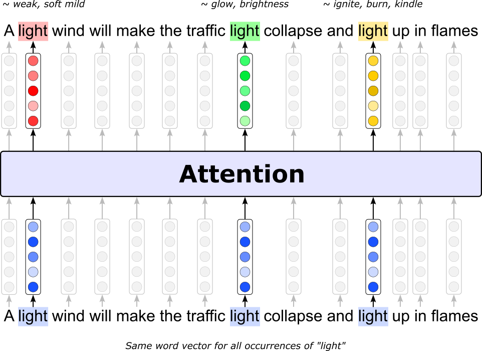
A light wind will make the traffic light collapse and light up in flames
Particularly with respect of the multiple occurrences of the token "light", all three occurrences of "light" represent a different syntactic function: first an adjective, then a noun, and lastly a verb. But even with respect to a single syntactic function, the same token may have (very) different meanings. For example, a traffic light is arguably a very different thing compared to a torch light — or just the noun "light" in a sentence like "I saw the light at the end of the tunnel". In short, representing all three occurrences with the same embedding vector would fail to capture these syntactic differences, and with that also the semantic differences.
So what we want is that the embedding vectors of tokens depend on the context, i.e., the sentence or paragraph a token occurs in). This is the goal of attention: it transforms (hence: Transformer architecture) the input token vectors such that they (hopefully) capture their (more) precise meaning depending on their surrounding context. The figure below illustrates the general goal using our previous example sentence, again focusing on the occurrences of the token "light". While the input uses the same token vector for "light", attention transforms these vectors such that they are more aligned with their actual meaning in the sentence.
So how does attention actually work: The core idea behind attention is the concept of alignment — the relationship between all tokens in a sequence to capture various types of relationships between the token2. These relationships help the model build a rich, contextual understanding of language. Examples of such relationships particularly include syntactic relationships (e.g., subject-verb agreement, modifiers and what they modify) and semantic relationships (e.g., coreference resolution, synonyms or paraphrases).
The alignment between two tokens are not calculated based on their initial embedding vectors; $d_{model}$ denotes the size of the input embedding vectors. This is because the same token can serve different purposes. Attention distinguishes three different embedding spaces:
Queries: The query embedding space can be thought of as a learned "search space" that represents what each token is trying to find or focus on in the sequence.
Keys: The key embedding space the content or features each token offers to the rest of the sequence. While queries express what a token is looking for, keys act like "descriptors" or "labels" of each token that say, "this is what I contain".
Values: The value embedding space in the attention mechanism represents the actual information that will be aggregated and passed on to the next layer — it is what gets transferred once a query decides which keys (i.e., tokens) to focus on.
To this end, attention uses three weight matrices — $\mathbf{W}_q$, $\mathbf{W}_k$, and $\mathbf{W}_v$ — to convert any input embedding vector to its corresponding query, key, or value vector. Compared to the $d_{model}$-dimensional space of the input embeddings, the query, key, and value spaces are typically of a lower dimension; we come back to that later when we talk about multi-head attention. Let's denote the sizes of the resulting query, key, and value vectors with $\mathbf{d}_q$, $\mathbf{d}_k$, and $\mathbf{d}_v$, respectively. As such we can define the tree weight matrices as:
In principle, the values for $d_q$, $d_k$, and $d_v$ may differ. However, in the Transformer architecture, all their values will always be identical. This means that we can assume that $d_q = d_k = d_v$. These three weight matrices contain all the learnable parameters of the attention mechanism. During training, these weight parameters get updated to learn better transformations of the input embeddings to their query, key, and value embeddings. In case of self-attention, where the goal is to capture the relationships between all tokens in the same sequence, we can define $\mathbf{Q}$/$\mathbf{K}$/$\mathbf{V}$ as the matrices containing all query/key/value vectors as follows:
Given $\mathbf{Q}$/$\mathbf{K}$/$\mathbf{V}$, attention is the defined as:
where the scaling factor $1/\sqrt{d_k}$ prevents the dot products between query and key vectors from becoming too large as the dimensionality of the query, key, and value spaces increases. The purpose of this scaling is to stabilize the softmax operation. Without scaling, large dot products (which grow with $d_k$) could result in very large exponentials in the softmax, causing it to produce extremely small gradients — making training harder and potentially unstable. Dividing by $d_k$ keeps the values in a range where softmax can function effectively, leading to more stable gradients and better convergence during training. This is also why this specific attention calculation is called scaled dot-product attention. The figure below visualizes the involved operations of the scaled dot-product attention using simple sequence containing $4$ tokens and $d_q = d_k = d_v = 6$.
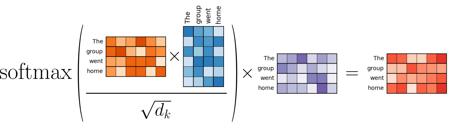
The key operation here is $\mathbf{QK}^\top$ as it computes the dot products (i.e., the alignments) between all tokens with respect to their query and key vectors. Intuitively, when two vectors point in the same direction, their dot product is large and positive; when they point in opposite directions, it's negative; and when they are orthogonal (perpendicular), the dot product is zero. This is because the dot product combines the lengths (magnitudes) of the vectors with the cosine of the angle between them, emphasizing how "aligned" they are. The figure below highlights this operation.
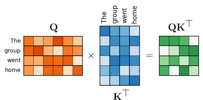
$\mathbf{Q}\mathbf{K}^\top$ now contains the attention scores for all pairs of tokens. The term "score" is commonly used to indicate that the values are, at least in principle, unbound since the dot product can range from $-\infty$ to $+\infty$. To ensure that the output vectors of the attention mechanism are of a similar magnitude, we need to normalize the (unbound) attention scores. More specifically, we have to normalize $\mathbf{Q}\mathbf{K}^\top$ such that all values in a row sum up to $1$ — the reason for this will be clear in a bit. To accomplish this, we can simply apply the softmax function to $\mathbf{Q}\mathbf{K}^\top$ — to each row in $\mathbf{Q}\mathbf{K}^\top$ to be more precise. The figure below illustrates this operation using a $\mathbf{Q}\mathbf{K}^\top$ matrix with some arbitrary attention scores.
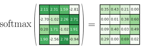
Note that the values of each row in the output matrix sum up to $1$.
The last step of the attention mechanism is to calculate the output as the product of the attention weights and the value vectors in $\mathbf{V}$. This multiplication means that the output embedding of a token (e.g., "group") is calculated as the weighted sum of all the embedding vectors in $\mathbf{V}$, including the token itself. The figure below illustrates this operation:
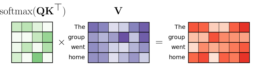
Notice here the importance of normalizing the rows in $\mathbf{Q}\mathbf{K}^\top$. Without it the values in the output vectors (red) may be of very different magnitudes compared to the value vectors (purple).
Summary: Attention transforms each input token vector $v$ by computing "some" aggregation of all other token vectors in the context of $v$; more specifically: the aggregation is the weighted sum of all value vectors in the $v$'s context, with the weights being derived from the pairwise similarity (usually based on the dot product) between the query and key vectors of all tokens. During training, the hope or expectation is that the model learn meaningful weight matrices $\mathbf{W}_q$, $\mathbf{W}_k$, and $\mathbf{W}_v$ — notice that these are the only parts with learnable parameters! — such that this transformation yields output token vectors better capturing the semantics of each token with respect to its current context.
Causal Masking
Essentially all Transformer-based LLMs on the market — GPT (OpenAI), LLaMA (Meta), Gemini (Google), Claude (Anthropic), Mistral, etc, — use decoder-only architecture. These models treat text generation as a language modeling problem, predicting the next token based on previous ones. Basically all popular Large Language Models (LLMs) — GPT (OpenAI), LLaMA (Meta), Gemini (Google), Claude (Anthropic), Mistral, etc, — are examples of decoder-only architectures. They are efficient for tasks like story generation, code completion, or question answering, where the context is part of the same sequence being generated rather than a separate input.
During training the LLM, the decoder receives the complete sequence. Without any considerations, the attention mechanism would compute all pairwise attention scores. This means that the output of the decoder at position $t$ would depend on all previous tokens as well as all subsequent tokens. In simple terms, during training, the decoder would be able to "look into the future". Thus, we have to ensure that each token only attends to previous tokens but not to subsequent tokens. We can accomplish this once more through masking, more commonly called causal masking because the mask enforces a cause-and-effect relationship in the sequence: each token can only "see" (i.e., attend to) previous tokens, not future ones. This preserves the causal structure necessary for autoregressive generation, where each output depends only on what has come before — not what comes after.
To illustrate this, let's consider self attention which is given a sequence of $5$ tokens (technically: tokens) as input. This means that after computing $\mathbf{QK}^\prime/d_k$, we get a $5\!\times\!5$ matrix containing all pairwise attention scores. Let's denote the matrix with the attention scores as $\mathbf{A}_{scores}$. However, as just motivated, we do not want to consider all those scores, but only the ones between each token and the ones preceding that token (and the token itself). To this end, we can define a diagonal matrix $\mathbf{A}_{causal}$ with $-\infty$ for all values above the diagonal:
Of course, like $\mathbf{A}_{scores}$, matrix $\mathbf{A}_{causal}$ has a size of $5\!\times\!5$ for our example. Applying this causal mask just means to add the attention scores on the mask, i.e., $\mathbf{A}_{masked} = \mathbf{A}_{scores} + \mathbf{A}_{causal}$. Since adding $-\infty$ to any value yields $-\infty$, the masked attenion scores will get a value of $-\infty$. After applying Softmax to $\mathbf{A}_{masked}$, i.e., $\mathbf{A}_{weights} = \text{Softmax}(\mathbf{A}_{masked})$, all masked attention scores in $\mathbf{A}_{masked}$ will be $0$ in $\mathbf{A}_{weights}$ — with all remaining values in each row of $\mathbf{A}_{weights}$ summing up to $1$. This effectively cancels out any attention between each token and their "future tokens" before computing $\mathbf{A}_{weights} \cdot \mathbf{Q}$.
Causal masking is essential for implementing the autoregressive behavior of an LLM because it prevents each token from attending to future tokens that are not yet available during generation. By restricting attention to the current and preceding tokens, causal masking ensures that the model predicts each next token using only information it could have seen at that point. This left-to-right structure is also what makes KV caching possible: once earlier tokens have been processed, their key and value representations remain valid and can be reused when generating subsequent tokens.
Important: By default, causal masking must also be applied during inference so that the model's generation setup remains consistent with the conditions under which it was trained. During training, each token is restricted from attending to future tokens, ensuring that its prediction is based only on preceding context. Applying the same restriction during inference preserves this autoregressive behavior. Without causal masking, tokens in the input sequence could attend to later tokens, allowing the model to use information that would not be available during ordinary left-to-right generation. Consequently, the same input sequence could produce different representations during training and inference, creating a mismatch between the two settings. As we will see, KV Caching implicitly performs causal masking, thus eliminating the need for adding $\mathbf{A}_{causal}$ when performing attention.
Lastly, a Transformer decoder typically consists of multiple stacked attention layers, with each layer refining the representation produced by the previous one. Early layers can capture local relationships and basic syntactic patterns, while deeper layers combine this information to model more complex dependencies, semantic relationships, and broader contextual structure. Stacking attention layers increases the model's expressive power and allows information to be integrated progressively across the sequence. This depth enables the decoder to transform simple token representations into rich contextual representations that are useful for predicting the next token. The figure below illustrates this idea.
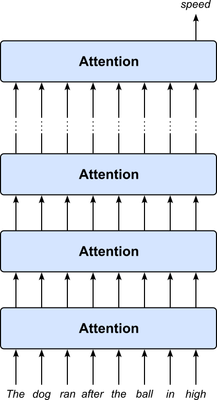
Side note: The previous figure shows a very simplified architecture of a Transformer decoder, focusing on the core idea of stacking multiple attention layers. However, the full architecture includes additional components such as fully connected layers, residual connections, batch normalization and dropout layers. Overall concept of a multilayer architecture remains the same, but it would make the figure unnecessary complex and would distract for key idea KV Caching and how it affects the attention mechanism or, more specifically, its implementation — later we modify this figure to show how KV caching integrates into this basic layered architecture for a direct comparison.
KV Caching Explained
In this section, we now take a deep dive into why and how KV Caching works. This includes that we show practical examples using from-scratch implementations of the attention mechanism with and without KV Caching for a direct comparison. Once we have a good understanding about its inner workings and characteristics, we analyze the memory footprint added by KV Caching in more detail.
Why it Works
Just by looking at the introductory example and the recap of how attention with causal masking works, you probably already got some idea why iteratively predicting the next token in an autoregressive manner involves repeated computations. However, it's worthwhile to really see what is going on under the hood to fully appreciate when and KC Caching helps. To this end, let's actually implement a basic version of the attention mechanism to first see how it works and behaves without any caching.
We start by implementing the scaled dot-product attention as defined above — that this, the method scaled_dot_product_attention() directly implements
but also includes the generation and application of a causal mask $\mathbf{A}_{causal}$ if causal=True; not all Transformer architectures implement attention with causal masking, so this implementation is — although not needed here — a bit more flexible. In general, it should be very straightforward to map each line of the method to the corresponding parts in the expression above. Note that we return the attention output as well as the attention weights. While the latter would not be needed to return in practice, we actually want to have a look at the weights later.
def scaled_dot_product_attention(Q, K, V, causal=False):
    seq_len, d_head = Q.shape

    # Compute scaled attention scores
    scores = Q @ K.transpose(1,0)
    scores = scores / np.sqrt(d_head)

    # Prevent positions from attending to future tokens
    if causal:
        mask = torch.triu(torch.ones(seq_len, seq_len, dtype=torch.bool), diagonal=1)
        scores = scores.masked_fill(mask, float("-inf"))

    # Normalize scores into attention weights
    attention_weights = torch.softmax(scores, dim=-1)

    # Compute the weighted sum of value vectors
    return attention_weights @ V, attention_weights
The method scaled_dot_product_attention() performs only the mathematical operations required to compute attention and contains no trainable parameters of its own. It receives the query, key, and value matrices ($\mathbf{Q}$, $\mathbf{K}$, and $\mathbf{V}$) as inputs. These matrices are obtained by transforming the input sequence embeddings using three learnable linear layers — which implement the three weight matrices $\mathbf{W}_q$, $\mathbf{W}_k$, and $\mathbf{W}_v$ — which independently project the embeddings into queries, keys, and values. Together, these linear projections and the scaled dot-product attention operation form an attention head.
In a complete Transformer, an attention layer typically contains multiple independent attention heads. Each head computes attention using its own learned projections, and the resulting outputs are subsequently combined. For understanding the basic mechanism of KV caching, however, it is sufficient to focus on a single attention head and examine how its key and value representations can be reused during autoregressive generation. The class AttentionHead implements this idea. Notice how this class only defines the three linear projects to map the input sequence to the respective sequences of query, key, and value vectors to get $\mathbf{Q}$, $\mathbf{K}$, and $\mathbf{V}$; and then calls scaled_dot_product_attention() to get the output of the attention head (again, we also return the attention weights for later inspection).
class AttentionHead(nn.Module):

    def __init__(self, d_model, d_head):
        super().__init__()
        self.d_model, self.d_head = d_model, d_head
        self.Wq = nn.Linear(d_model, d_head)
        self.Wk = nn.Linear(d_model, d_head)
        self.Wv = nn.Linear(d_model, d_head)

    def forward(self, sequence, causal=False):
        Q, K, V = self.Wq(sequence), self.Wk(sequence), self.Wv(sequence)
        # Compute scaled-dot product attention and return result and attenion weights
        return scaled_dot_product_attention(Q, K, V, causal=causal)
Side note: Transformer architectures generally distinguish between self-attention and cross-attention. Self-attention allows tokens within the same sequence to attend to one another, whereas cross-attention enables one sequence—typically a decoder—to attend to representations produced by an encoder. In encoder–decoder models, cross-attention therefore provides the connection between the encoder and decoder. Since we focus on decoder-only architectures commonly used for LLMs, no separate encoder output is available or required, and cross-attention is unnecessary. Accordingly, our implementation of an attention head considers self-attention only.
To show how our attention head works, we need some example data. For this, we first have to specify two core parameters
- $d_{model}$: the size of the input embeddings
- $d_{head}$: the size of the query, key, and value vectors; recall that we assume $d_q = d_k = d_v$
Although not important here, the values of $d_{head}$ is typically set to $d_{head} = d_{model} / n_{heads}$, where $n_heads$ is the number of attention heads in the attention layer. In the code cell, we set $d_{model} = 12$ and $d_{head} = 6$ which implies that we assume having two attention heads, i.e., $n_{heads} = 2$. Again, for our examples here, the actual values are not important, but we do limit ourselves to small values for $d_{head}$ to ease the readability of the results.
d_model, d_head = 12, 6
Regarding the data — since our goal is not to predict anything meaningful, we can simply generate a list of, say, five input embedding vectors. Of course, we have to make sure that these embedding vectors have the correct size of $d_{model}$ to serve as valid input to the attention head.
torch.manual_seed(42)

embeddings = [ torch.rand(1, d_model) for _ in range(5) ]
We can now create an instance of our AttentionHead. Note that we also set a random seed here to ensure that the weight matrices and biases of our three linear projection layers are always initialized the same way for consistent outputs.
torch.manual_seed(42)

attention = AttentionHead(d_model, d_head)
We have the attention had; we have the data. We can now explore how attention behaves when generating text in an autoregressive manner. Since we only consider the attention head — and therefore cannot really predict any next token — the code cell below works as follows: starting with an empty sequence, we iteratively each embedding vector to the sequence and pass it to that attention heads to get the output and attention weights. This mimics the step where we append the last predicted token (i.e., its embedding vector) to the input sequence. Again, this works here because we are not interested in the actual values. In short, the code cell below yields the output after each iteration.
# Initialize empty sequence
sequence = torch.empty((0, d_model))

with torch.no_grad():
    for step, emb in enumerate(embeddings):
        # Add next embedding vector to current sequence
        sequence = torch.vstack((sequence, emb))
        # Compute attention head output
        output, weights = attention(sequence, causal=True)
        # Convert PyTorch tensor to NumPy array
        #output = output.detach().numpy()
        # Display output
        print(f"\nOutput of attention head after Step {step+1}")
        draw_matrix(output, decimals=3)
Output of attention head after Step 1
Output of attention head after Step 2
Output of attention head after Step 3
Output of attention head after Step 4
Output of attention head after Step 5
Most obviously, the size of the output increases by one vector in each iteration. This is simply because the input increases each time because we add the most recent token, and the output size of the attention head is the same as the input size.
The more important observation, however, is that the output of the $t$-th iteration is the same as the output of the $(t\!-\!1)$-th iteration only with the newly added vector caused by the extended input. Keep in mind that the outputs were computed completely independently in each iteration. Furthermore, recall that the output of attention is either passed to the next attention layer or some output layer. This essentially means that an attention layer passes the same $(t\!-\!1)$ output vectors that the subsequent layer has already seen before. In simple terms, we do not tell the next layer anything new about the past.
Side note: In practice, the initial input is typically not a single token but a complete prompt, i.e., a potentially long sequence of tokens. For this example, we basically assume that the prompt is a single token, but only to keep the example small and easy to read. We could have started with an initial sequence of, say, $10$ tokens. The overall insight would be exactly the same, only that the example output would be much larger and thus less easy to comprehend.
We can make a similar observation when looking not at the output but at the attention weights. In the code cell below, we perform the exact same loop as before only that we now show the matrix of attention at the end of each iteration.
# Initialize empty sequence
sequence = torch.empty((0, d_model))

with torch.no_grad():
    for step, emb in enumerate(embeddings):
        # Add next embedding vector to current sequence
        sequence = torch.vstack((sequence, emb))
        # Compute attention head output
        output, weights = attention(sequence, causal=True)
        # Convert PyTorch tensor to NumPy array
        #output = output.detach().numpy()
        # Display output
        print(f"\nAttention weights after Step {step+1}")
        draw_matrix(weights, decimals=3)
Attention weights after Step 1
Attention weights after Step 2
Attention weights after Step 3
Attention weights after Step 4
Attention weights after Step 5
Again, notice how the matrix with the attention weights systematically "grows" by a new row and column — remember that the attention matrix is a square matrix with its size representing the length of the sequence since the attention weights reflect the alignment between all pairs of tokens in the sequence. This means, for example, when predicting the $6$th/$7$th/$8$th/... token, the attention weight between the $3$rd and $5$th token will always be the same. Otherwise we would not see the identical outputs for past iterations.
Important: The attention paid to a token remains the same across positions only because of causal masking. Without causal masking, each token would attend to an increasingly longer sequence, requiring us to compute the softmax over a growing vector and consequently producing different attention weights at each position. Causal masking blocks the attention between a token and any tokens that follow it in the sequence. As a result, each token attends only to the same preceding context, so the relevant attention weights remain unchanged as the sequence continues. You can actually see this for yourself if you run the previous two code snippets with causal=False, thus omitting causal masking. In this case, both the outputs and attention matrices will always look different with respect to all values.
Basic Idea
We have just seen using a concrete example how the attention output "simply grows" every time we predict the next word. To better appreciate later where KV Caching improves inference speed, consider the figure below that illustrate the basic attention computation $\text{Attention}(\mathbf{Q}, \mathbf{K}, \mathbf{V})$; in this example, we assume an input sequence length of $6$ and a more practical size of $64$ for the query, key, and value vectors, in $\mathbf{Q}$, $\mathbf{K}$, and $\mathbf{V}$. Note that $\mathbf{QK}^\top$ represents the matrix with attention, and the grey entries reflect the ignored weights after causal masking.

Given this figure it is easy to see that we have to perform computations that we already did before. For example, assuming we started with an initial context of length $3$, we computed the dot product between the first query vector and the first key vector already three times — to predict the 4th, 5th, and 6th token. More specifically, given a context of length $t$, to predict the next token, we need the following information
- All key vectors for the previous tokens $w_1$, $w_2$, $w_{t-1}$ [which we also needed in the previous iteration!]
- All value vectors for the previous tokens $w_1$, $w_2$, $w_{t-1}$ [which we also needed in the previous iteration!]
- The query, key, and value vector for token $w_t$
This makes the idea behind KV Caching very clear: Since we always need the same key and value vectors from the previous iteration, the idea is to simply cache seen query and value vectors instead of always recomputing them. Together with the fact that we only need the query vector for token $w_t$ — instead of also the query vectors of all previous tokens — to predict the next token $w_{t+1}$, the attention computation simplifies as shown below:

where the blue vectors indicate the key and value vectors taken from the cache, which can significantly speed up the attention computation. Notice that the output attention output is now only a single vector reflecting the output of the most recent iteration. Recall, however, that we only need to pass on this vector since any subsequent layer will have past vectors in its own cache. The figure below extends the previous example illustrating a Transformer decoder with multiple attention layers, but with a cache added to each attention. The grey arrows indicate the one-time passing of past outputs from the preceding layer that have been added to the cache.
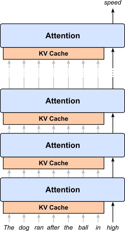
This figure also already hints at the main challenge that comes with KC Caching: the additional memory requirements. Not only do we typically attach a cache to each attention layer, the cache also grows during the text generation as each newly predicted token causes a new key and value vector to be added to the cache — again, at each layer! We look into the overall footprint of KV Caching and which parameters affect it in more details later, after we have implemented and tested a simple version of attention with KV Caching.
Toy Implementation
Implementing a KV cache is relatively straightforward because it mainly involves maintaining two lists: one for the key vectors and one for the value vectors computed for previously processed tokens. During each generation step, the newly computed key and value vectors are appended to these lists and reused in subsequent attention calculations. This avoids recomputing keys and values for the entire preceding sequence, while requiring only a simple mechanism for storing and retrieving the accumulated states. The main implementation challenge is therefore not the caching logic itself, but managing the cache’s growing memory footprint efficiently.
To make this more practical, the class KVCache in the code cell below implements a minimal example of a KV cache. The two class attributes keys and values represent the two lists (more specifically: PyTorch tensors) that hold all past key and value vectors. The update() method either initializes the cache in case of the first vectors — recall that the initial input may have many tokens — or adds the current vectors to the cache. The reset() method is simply to empty the cache; we also overwrite the __len__() method to conveniently get the size of the cache in terms of the number of key vectors; the number of key and value vectors in the cache is always expected to be the same.
class KVCache:

    def __init__(self):
        self.keys, self.values = None, None

    def update(self, new_key, new_value):
        # If the cache is empty, initialize with first key and value vectors
        if self.keys is None:
            self.keys, self.values = new_key, new_value
        # Otherwise, add key and value vector to cache
        else:
            self.keys = torch.cat([self.keys, new_key], dim=0)
            self.values = torch.cat([self.values, new_value], dim=0)
        # Return updated cache; convenient for later use
        return self.keys, self.values

    def reset(self):
        self.keys, self.values = None, None

    def __len__(self):
        if self.keys is None:
            return 0
        return self.keys.size(1)
We can now modify our implementation of the attention head to make use of a KV cache; see the AttentionHeadKV in the code cell below. Notice that the __init__() remains unchanged since we pass the cache as an argument of the forward() method. Not making the cache a class variable keeps the class leaner and adds flexibility. The class, more specifically, the forward() method must handle three main cases:
- Training: KV caching is only applicable during inference, so we must ignore it during training; we specify this by not passing any cache, i.e.,
kv_cache=None. In this case,sequencecontains one or more long lists of tokens (depending on the batch size) - Inference (initial prompt): Here we pass a cache as an argument but the cache is still empty. Since the prompt will be a whole sentence of paragraph,
sequencewill again be a list of tokens; let's assume a batch size of $1$ for inference here to keep things simple. Thus, for the initial tokens, we do need apply causal masking - Inference (predicting next word): In the main iterative step,
sequenceis now a single vector representing the last predicted token. Note that when we update the cache with this tokens key and value vector, theupdate()method conveniently returns the newKandVwe can then pass to thescaled_dot_product_attention()method.
In short, switch KV Caching on or off by either passing an instance of the KVCache class (during inference) or None (during training). Apart from the distinction between training and inference, we also have to consider the special case of the initial input during inference.
class AttentionHeadKV(nn.Module):

    def __init__(self, d_model, d_head):
        super().__init__()
        self.d_model, self.d_head = d_model, d_head
        self.Wq = nn.Linear(d_model, d_head)
        self.Wk = nn.Linear(d_model, d_head)
        self.Wv = nn.Linear(d_model, d_head)

    def forward(self, sequence, causal=False, kv_cache=None):
        Q = self.Wq(sequence)
        new_K = self.Wk(sequence)
        new_V = self.Wv(sequence)

        if kv_cache is not None:
            had_cached_tokens = len(kv_cache) > 0
            K, V = kv_cache.update(new_K, new_V)
            # During inferene, the new token may attend to all cached tokens.
            # Causal masking is needed only when processing the initial sequence.
            causal = causal and not had_cached_tokens
        else:
            K, V = new_K, new_V

        output, weights = scaled_dot_product_attention(Q, K, V, causal=causal)

        return output, weights
To see how this works, we first create an instance of the modified attention class AttentionHeadKV as well as of class AttentionHeadKV. We set the same random seed again to meaningfully compare the output with the previous one we got from the attention class without KV Caching.
torch.manual_seed(42)

attention_kv = AttentionHeadKV(d_model, d_head)
cache = KVCache()
Similar to the previous example, we can now mimic autoregression text generation using a simple loop where we iteratively add the next token vector to the input sequence. Again, we assume that our prompt, i.e., the initial input, is a single token to keep the output simple and in line with the example without using KV Caching (see above). Notice how the code below treats the first input separately to initialize the cache; which includes the need for causal masking. After that, in the loop, we use and update the cache as part of the attention computation.
cache.reset()

with torch.no_grad():
    # Initial prompt: populates the cache
    output, _ = attention_kv(embeddings[0], causal=True, kv_cache=cache)
    # Display output
    print(f"\nOutput of attention head after Step 1")
    draw_matrix(output.numpy(), decimals=3)

    for step, emb in enumerate(embeddings[1:]):
        output, _ = attention_kv(emb, causal=False, kv_cache=cache)
        # Display output
        print(f"\nOutput of attention head after Step {step+2}")
        draw_matrix(output.numpy(), decimals=3)
Output of attention head after Step 1
Output of attention head after Step 2
Output of attention head after Step 3
Output of attention head after Step 4
Output of attention head after Step 5
If you compare this output with the one without KV Caching you will notice that we now only get a single vector reflecting the output for the last token. Since we use the same random seeds to initialize the attention head (i.e., the weight matrices and bias vectors of three projection layers), each vector matches the last row in the growing output matrix when not using KV Caching. Of course, we did not lose any information since we already know that past output vectors do not change when predicting the next word.
For the sake of completeness, we run the same code again, but only this time showing the attention weights after each iteration.
cache.reset()

with torch.no_grad():
    # Initial prompt: populates the cache
    output, weights = attention_kv(embeddings[0], causal=True, kv_cache=cache)
    # Display output
    print(f"\nAttention weights head after Step 1")
    draw_matrix(weights.numpy(), decimals=3)

    for step, emb in enumerate(embeddings[1:]):
        output, weights = attention_kv(emb, causal=False, kv_cache=cache)
        # Display output
        print(f"\nAttention weights head after Step {step+2}")
        draw_matrix(weights.numpy(), decimals=3)
Attention weights head after Step 1
Attention weights head after Step 2
Attention weights head after Step 3
Attention weights head after Step 4
Attention weights head after Step 5
Since we only need the query vector for the last token, $\text{Softmax}(\mathbf{QK}^\top)$ will naturally also be just a single vector — after all, we only need this single attention vector to compute the single output vector. But once again, output vectors after each iteration match the last row in the growing attention matrix when not using KV Caching.
Memory Tradeoff
KV caching significantly speeds up autoregressive inference by avoiding repeated computation of keys and values for previously processed tokens. However, this speed-up comes at the cost of additional memory usage. The key-value cache must typically be maintained for every attention layer, and its size increases as more tokens are generated. Consequently, the KV cache can become a substantial part of the model’s memory footprint, especially for large models, long sequences, or large batches. More specifically, the additional memory required for KV Caching depends on the following parameters
- $t$: sequence length (which grows over time!)
- $b$: batch size (if the LLM generates multiple outputs in parallel)
- $n_{layers}$: number of decoder layers/blocks (i.e., attention layer) in the complete decoder
- $n_{heads}$: the number of attention heads in a single attention layer
- $d_{head}$: the size of the query, key, and value vectors; typically $d_q = d_k = d_v$
- $p$: precision of the weights (e.g., float16 vs float32)
Considering that we need to store both key and value vectors, the total memory required can be computed as:
In practice, of course, some more memory will be needed for any kind of overhead data (e.g., additional data structures for indexing).
To give a concrete example, let's consider trying to run a small pretrained LLM with $7$ Billion parameters locally, say LLaMA 2 7B. Assuming a precision for the weights of $p=2$ bytes (float16), just the model alone will require 14-16 GB of memory. At the time of writing (September 2026) 16 GB of VRAM has become the standard for many mid/upper-range consumer GPU cards. However, now we want to speed up inference by deploying KV Caching. For the memory calculation let's assume the following values for the relevant parameters — the model parameters do in fact match the ones of the LLaMA 2 7B model:
- $t = 500$ (i.e., we cap the maximum number of output tokens)
- $b = 32$: batch size (if the LLM generates multiple outputs in parallel)
- $n_{layers} = 32$: number of decoder layers/blocks (i.e., attention layer) in the complete decoder
- $n_{heads} = 32$: the number of attention heads in a single attention layer
- $d_head =128$: the size of the query, key, and value vectors; typically $d_q = d_k = d_v$
- $p$: precision of the weights (e.g., float16 vs float32)
Thus, if we plug in those numbers, we get:
This means that for these numbers, and considering some overhead, the memory footprint of running the model would increase by around 50% when using KV Caching. While consumer GPU cards with 24 GB VRAM or even above are available, they are significantly more expensive. That being said, when running a pretrained locally at home, there is generally no need to generate multiple outputs in general. Thus, if we assume a batch size of $b=1$, the memory footprint quickly drops around 250 MB (again, allowing for some overhead). Still, for large frontier models running on huge computing clusters and serving many users at the same time, the batch size remains a critical parameter
Due to the benefits of KV Caching in terms of improved inference speed but also its significant impact on the overall memory footprint, a wide range of strategies have been proposed to reduce the amount of additional memory required for KV Caching. Below, we briefly outline some of the more popular strategies — but a detail discussion is beyond the scope of this notebook
Quantization & Precision Reduction. Quantization and precision reduction compress the KV cache by storing key and value tensors in lower-bit numerical formats (like FP8, INT8, or INT4) instead of standard 16-bit floating points (FP16/BF16). The system dynamically calculates scaling factors to fit continuous floating-point values into smaller representations before saving them to GPU memory, cutting cache memory requirements by 50% to 75%. However, aggressive quantization can introduce precision loss on tasks requiring high numerical precision or complex reasoning. Additionally, if the target hardware lacks native instruction support for low-precision tensor operations, dequantizing values on-the-fly back to FP16 can introduce compute latency that reduces overall throughput.
Eviction & Pruning (Token Dropping). The goal is to manage the growth of the KV cache by permanently discarding less important token key-value pairs based on importance metrics like cumulative attention scores or positional recency. Instead of storing every historical token indefinitely, the system maintains a fixed-size memory budget that prioritizes critical information. This shifts KV cache memory overhead from scaling, in principle, endlessly to staying strictly bounded or constant. In practice, this is implemented using algorithms like StreamingLLM (combining initial sink tokens with a local sliding window) or H2O (retaining historically high-attention "heavy hitter" tokens). The primary drawback is irreversible context loss: if a pruned token suddenly becomes relevant later in a complex dialogue or multi-step reasoning task, the model cannot retrieve it and may hallucinate. Furthermore, calculating token importance scores and continually reorganizing memory buffers introduces extra computational overhead during decoding.
Memory Allocation & System-Level Optimizations. System-level optimizations for KV caching eliminate physical VRAM waste without altering model accuracy or pruning tokens. Standard serving frameworks traditionally pre-allocate large, contiguous memory blocks based on maximum expected sequence lengths, resulting in up to 60% memory waste from internal and external fragmentation. System-level approaches solve this by applying operating system memory management concepts to divide key-value states into small, fixed-size blocks allocated strictly on demand as new tokens are generated. Technologies like PagedAttention manage dynamic block lookup tables to store sequences in non-contiguous physical GPU pages, while supporting features like copy-on-write page sharing for common prompt prefixes. While this approach preserves full context precision and drastically boosts server throughput by enabling larger batch sizes, it comes at the cost of added system complexity. Managing non-contiguous memory requires custom attention CUDA kernels, introduces minor lookup overhead, and can hit hardware transfer bottlenecks if swapping pages between GPU VRAM and CPU system memory.
Architecture & Attention Variants. Standard Multi-Head Attention maintains a separate key and value head for every query head, causing cache requirements to scale heavily. Variants alter this balance: Multi-Query Attention (MQA) shares a single KV head across all query heads, Grouped-Query Attention (GQA) groups query heads to share a smaller subset of KV heads, and Multi-Head Latent Attention (MLA) compresses keys and values into a low-dimensional latent vector before caching. By decoupling KV heads from query heads, these designs shrink the per-token KV cache footprint, drastically reducing memory bandwidth bottlenecks during decoding and allowing for higher throughput and batch sizes. However, these architectural changes are baked into the model weights and require pre-training or costly fine-tuning to adopt. Additionally, aggressive sharing (like MQA) can slightly degrade model capacity on complex reasoning tasks, while advanced approaches like MLA rely on specialized CUDA kernels to re-project latent vectors efficiently during inference.
Summary
This notebook provided a comprehensive exploration of Key-Value (KV) Caching, a foundational technique for accelerating autoregressive text generation in Transformer-based LLMs. By walking through the mechanics of the self-attention mechanism, the notebook clearly demonstrated why standard token-by-token generation is computationally inefficient when executed naively. It established how autoregressive decoding repeatedly recalculates identical Key and Value tensor representations for historical tokens, creating a severe operational bottleneck as context length grows.
To overcome this bottleneck, the notebook detailed both the theoretical framework and practical implementation of KV Caching. It illustrated how storing the intermediate key and value vectors of past tokens in GPU memory enables the model to process only the single newest token at each decoding step. By retrieving pre-computed vectors from the cache rather than recalculating them from scratch, KV Caching dramatically reduces redundant matrix multiplications, transforming inference latency and turning slow, step-by-step decoding into a highly responsive process.
However, the notebook also underscored the critical trade-off inherent to this approach: its substantial memory footprint. Unlike fixed model parameters, the KV cache grows dynamically and linearly with context length, batch size, number of layers, and hidden dimensions. As context windows expand into tens or hundreds of thousands of tokens, the memory required to maintain the cache can easily exceed the memory needed for the model weights themselves, leading to severe VRAM fragmentation, restricted batch sizes, or out-of-memory errors on serving hardware.
In conclusion, while KV Caching has rightfully become an indispensable staple for efficient LLM inference, managing its aggressive memory demands remains a vital challenge. As long-context applications continue to push the boundaries of modern AI, pairing standard KV Caching with advanced memory optimizations (such as low-bit quantization, structural attention variants, token eviction, and paged memory allocation) is essential for sustaining high-throughput, cost-effective model deployment.