Disclaimer: This Jupyter Notebook contains content generated with the assistance of AI. While every effort has been made to review and validate the outputs, users should independently verify critical information before relying on it. The SELENE notebook repository is constantly evolving. We recommend downloading or pulling the latest version of this notebook from Github.

Attention & Multi-Head Attention

In the Transformer architecture, the attention mechanism is the core component that enables the model to process sequences without relying on recurrence or convolution. Self-attention allows each element of a sequence (like each word in a sentence) to consider and weigh all other elements in the sequence simultaneously when producing an output representation. For every word, the model computes a weighted sum of all other words' representations, where the attention weights reflect how relevant each word is to the current word being processed.

The primary purpose of attention in Transformers is to capture dependencies between words or elements, regardless of their distance in the sequence. Traditional models like RNNs or LSTMs struggled with long-range dependencies because information from distant positions had to pass through many steps, leading to degradation or loss of information. Self-attention overcomes this by enabling direct interaction between all pairs of elements, allowing the model to quickly learn relationships between distant and nearby tokens alike. This is especially powerful in tasks like language modeling, translation, and text summarization where context from the entire sequence is often necessary.

What makes attention in Transformers particularly useful is not only its ability to capture global dependencies but also its computational efficiency and scalability. Since self-attention can be computed in parallel across all positions (unlike sequential RNNs), Transformers can take advantage of modern hardware (like GPUs and TPUs) to train on massive datasets much faster. Furthermore, mechanisms like multi-head attention — where multiple sets of attention computations run in parallel — allow the model to capture different types of relationships simultaneously, enriching its representational power.

Understanding attention in Transformers is crucial because it lies at the heart of nearly all state-of-the-art models in natural language processing and beyond. Models like BERT, GPT, T5, and even newer architectures in computer vision and audio processing all rely on variations of this mechanism. Grasping how self-attention works gives deep learning practitioners the ability to design, interpret, and improve models that are now central to modern AI applications.

Setting up the Notebook

Make Required Imports

This notebook requires the import of different Python packages but also additional Python modules that are part of the repository. If a package is missing, use your preferred package manager (e.g., conda or pip) to install it. If the code cell below runs with any errors, all required packages and modules have successfully been imported.

import torch
import torch.nn as nn

Preliminaries

Before delving into the inner works of attention and multi-head attention, there are a few preliminary comments to outline the scope of this notebook:

• Attention is a general concept and in fact has been popularized in the context of Recurrent Neural Networks (RNNs). However, here we introduce attention and multi-head attention as introduced and generalized in the original Transformer paper "Attention is all you Need". However, this does not change the underlying purpose and ideas behind attention.

• Since we focus on the original Transformer, we assume text as input — in fact, we consider a machine learning task as an example use case throughout the notebook (see below). To make all visualizations, examples, and descriptions easier to understand, we assume that any input text is tokenized into proper words. Note that practical Transformer-based models typically rely on subword-based tokenizers (e.g., Byte-Pair Encoding, WordPiece).

With these clarifications out of the way, let's get started...

---

Motivation & Intuition

Recall that words need to be encoded as vectors to serve as input for neural network architectures because neural networks are designed to process numerical data, not symbolic text. A word in its raw form — like "apple" or "computer" — is just a sequence of characters without any inherent numeric meaning that a machine can interpret mathematically. To make text data usable for computation, we must transform these words into a form that the network's matrix operations and optimization algorithms (like gradient descent) can work with. Vectors, which are arrays of numbers, provide this bridge between symbolic language and numerical computation.

Although not crucial for our discussion here, recall that we favor word vectors (or word embeddings) that map words into a continuous vector space where similar words with similar meanings are mapped to similar vectors. These vector representations are crucial for neural networks to exploit similarities, analogies, as well as generalize patterns across language data. If the model understands that similar words have similar vectors, it can apply what it learned about one word to another related word, improving efficiency and performance in tasks like classification, translation, and question answering. Without this numerical structure, the network would have no way to infer that similar-sounding sentences or synonyms are related, leading to poor generalization and ineffective learning.

However, mapping an individual word to its embedding vector has its limitations. In natural languages, the same word may have different meanings or different syntactic functions depending on the context, i.e., the phrase or sentence the word occurs in. For example, consider the following sentence:

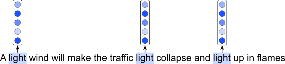
A light wind will make the traffic light collapse and light up in flames

Particularly with respect of the multiple occurrences of the word "light", what are the issues that arise when encoding the same word with the same embedding vector:

• All three occurrences of "light" represent a different syntactic function: first an adjective, then a noun, and lastly a verb. Representing all three occurrences with the same embedding vector would fail to capture these syntactic differences, and with that also the semantic differences.
• Even with respect to a single syntactic function, the same word may have (very) different meanings. For example, a traffic light is arguably a very different thing compared to a torch light — or just the noun "light" in a sentence like "I saw the light at the end of the tunnel". Again, using the embedding vector for each occurrences of "light" would limit a model's capacity to better capture the context-dependent semantics of words.

The image below illustrates the this approach of encoding the same word with the same embedding vector; of course, all words in the sentence would be encoded as vector, but for clarity, we focus only on the vectors for the three occurrences of "light" in our example sentence.

Side note: At least in the Transformer architectures, the embedding vectors would strictly speaking not be exactly the same for the same words in a sentence. This is because positional embedding vectors are added to the word embeddings to inject information about the position or order of words in a sequence, since these models lack inherent sequence awareness. They enable the model to capture the relative or absolute position of words, which is crucial for understanding context and meaning in language. Without them, the model would treat input tokens as an unordered set. However, the components of the final embedding vectors that capture the semantic words (and not the position) are still the same for the same words.

So what we want is that the embedding vectors of words depend on the context (e.g., the sentence or paragraph a word occurs in) as well as the word order (this is where the positional embeddings come in). Again, we can illustrate this goal using our example sentence where now each occurrence of "light" is associated with a different embedding vector.

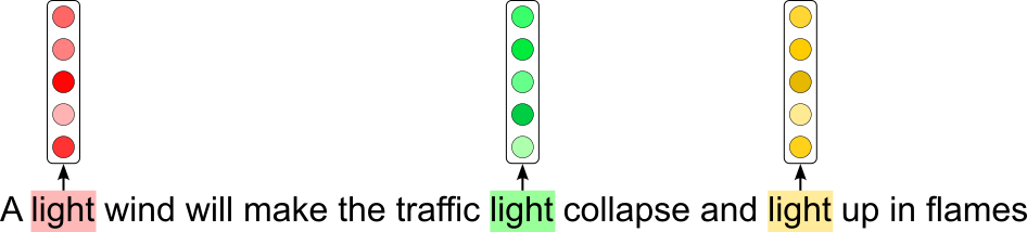
The goals is that these contextualized embedding vectors better capture the semantic meaning of the word; for example:

• "A light wind": here the embedding vector for "light" should be similar to the embeddings of other adjectives such as "soft", "mild", or "weak".

• "the traffic light": ideally, the embedding for "light" should be similar to other objects (i.e., nouns) that give of light; this may include "lamp", "street light", "lamp pole", and similar concepts.

• "light up in flames": in this context, the embedding for "light" should arguable similar to verbs such as "ignore", "burn", or "kindle"

There are different approaches towards contextualized word embeddings. One of the first for training such word embeddings was ELMo (Embeddings from Language Models) based on Recurrent Neural Networks (RNNs). More specifically, ELMo trains a bidirectional LSTM (Long Short-Term Memory) network on a large corpus with a language modeling objective — meaning it learns to predict both forward and backward sequences of words. This bidirectionality allows ELMo to capture both past and future context for each word in a sentence. The resulting word representations from ELMo are a combination of the internal states from all layers of the bidirectional LSTM, weighted depending on the task at hand. Because these embeddings dynamically change based on surrounding words, they can better capture word sense disambiguation — for example, the word "light" will have different embeddings in the sentences "traffic light" and "candle light".

However, since ELMo embeddings are RNN-based their training and effectiveness to generate good contextualized word embeddings are restricted due to inherent challenges associated with RNNs. Firstly, RNNs — including variants such as LSTMs and GRUs — process sequences sequentially. This sequential nature makes it difficult to parallelize computations, leading to slower training and inference times compared to models that process sequences more efficiently. And secondly, although ELMo captures contextual information bidirectionally, RNNs have difficulty modeling long-range dependencies effectively — information from distant words may degrade or be forgotten as the sequence progresses, limiting the quality of context representation for long sentences.

Addressing these two core issues was the main motivation behind the Transformer architecture, and the fundamental concept facilitating the generation of contextualized word embeddings is attention. Later, we will cover in detail how attention calculates contextualized word embeddings in such a way that (a) the required computations can easily be parallelized and (b) the distances between words no longer matter. At the moment, on a very high level, attention — or attention head (common terminology in the transformer architecture) — isa network component that takes in a sequence of embedding vectors and returns a sequence of recalculated embedding vectors. The figure below illustrates this idea of an attention head:

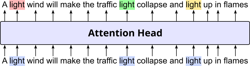
Again, the embedding vectors for all he words will be recalculated, but the figure only highlights this idea for the three occurrences of the word "light".

In general, an attention head aims to capture syntactic relationships (e.g., subject-verb agreement, modifiers and what they modify) and semantic relationships (e.g., coreference resolution, synonyms or paraphrases) between words. This includes that even the same pair of words may form different relationships. To capture different types of such relationships in parallel, the Transformer architecture employs more than one attention head in parallel for the same input sequence(s). All parallel attention heads are combined into a single network layer called multi-head attention. The figures below visualizes this idea combining 3 attention heads into a multi-head attention layer.

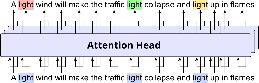
Despite having multiple attention heads, the output of the multi-head attention layer is still a single recalculated embedding vector for each input word. This is done by combining the outputs of all attention heads. How this and all other involved operations are done is the subject of the next section.

---

Multi-Head Attention: A Deep Dive

The concept of attention has been generalized and adopted for different architectures. In this notebook, focus on the application of attention within the original Transformer architecture. Strictly speaking, the attention has already been introduced as an extension for Recurrent Neural Networks (RNNs). However, as a fundamental concept, attention has been fleshed out and more generalized in the Transformer architecture. In fact, attention — and its extended implementation as multi-head attention — is the heart of the Transformer.

Let's look more closely how attention and multi-head attention works in detail by defining, visualizing, as well as implementing all the involved calculations. Throughout this notebook, we will be using a machine translation task based on the Transformer architecture as an example setup. More specifically, we assume an English-to-German translation task, and consider the following single training sample:

The group went home (English) $\Rightarrow$ Die Gruppe ging nach Hause (German)

Machine translation is commonly considered a sequence-to-sequence task that relies both the encoder and decoder of the Transformer architecture. This has the advantage that we can capture both instances of attention: self-attention and cross-attention — we will cover their difference in full detail later. In contrast, classification or sequence labeling tasks utilize only the encoder, while many language modeling tasks utilize only the decoder of the Transformer architecture.

Regarding formal definitions, we will be using the same notations as the original Transformer paper Attention is all you Need for consistency. The first important parameter we need to introduce is ${d_model}$ as follows:

• $\large d_{model}$: size of input embedding vectors as well as the output embedding vectors of a multi-head attention component

In practical, large-scale Transformer architectures, the size of $d_{model}$ typically ranges from several hundreds to several thousands. Just to give some examples, the table below shows the $d_model$ values for a few popular Transformer architectures.

Model	Architecture	$d_{model}$
BERT-base	encoder-only	768
BERT-large	encoder-only	1,024
GPT-3 Curie	decoder-only	2,048
GPT-3 Davinci	decoder-only	12,288
LLaMA 1/2/3 (7B)	decoder-only	4,096
LLaMA 1/2/3 (13B)	decoder-only	5,120
LLaMA 1/2/3 (70B)	decoder-only	8,192
T5-Base	encoder-decoder	768
T5-Large	encoder-decoder	1,024
BART-Base	encoder-decoder	768
BART-Large	encoder-decoder	1,024

To illustrate the calculations behind attention and multi-head attention, we naturally use a much smaller embedding size. More specifically, we set $d_{model} = 12$ throughout the rest of the notebook. As such, the figure below visualizes the input embedding tensor $\mathbf{X}$ of the English sentence "The group went home" with each of the 4 words represented by a 12-dimensional word embedding vector:

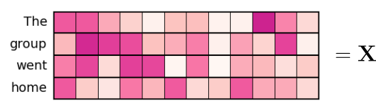
The tensor for the German sentence "Die Gruppe ging nach Hause" naturally looks similar, only with 5 rows instead of 4.

Since we also implement attention and multi-head attention from scratch, we can also define some basic variables as well as random embedding tensors for our English and German sentences. Notice that we assume a batch size of 1. Again, this just to keep the examples and corresponding illustrations simple. However, implementations will support batches containing more than one training sample.

batch_size, d_model = 1, 12
seq_en_len, seq_de_len = 4, 5

input_en = torch.rand(batch_size, seq_en_len, d_model)
input_de = torch.rand(batch_size, seq_de_len, d_model)

Note that we do not care about the actual values of the embedding vectors here, as we are only interested in the required calculations.

Scaled Dot-Product Attention

The core idea behind attention is the concept of alignment — the relationship between words within the same sequence (i.e., self-attention) or across different sequences (i.e., cross-attentions). This allows the model to dynamically focus on relevant parts of a sequence. In self-attention, alignment aims to capture various types of relationships between words in a sequence. These relationships help the model build a rich, contextual understanding of language. Examples of such relationships particularly include syntactic relationships (e.g., subject-verb agreement, modifiers and what they modify) and semantic relationships (e.g., coreference resolution, synonyms or paraphrases).

In contrast, in cross-attention and in the context of machine translation, the purpose is to align the word(s) from the source language to the matching word(s) in the target language. Other common relationships include lexical substitution or paraphrasing (i.e., when a target word is not a direct translation but a paraphrase or semantic equivalent), reordering or word order mapping for languages that significantly differ in their syntax (e.g., subject-verb-object order vs. subject-object-verb order), and others.

Embedding Transformation

The alignment between two words are not calculated based on their initial embedding vectors (i.e., example tensor $E$, see above). This is because the same word can serve different purposes. Attention distinguishes three different embedding spaces:

• Queries: The query embedding space can be thought of as a learned "search space" that represents what each token is trying to find or focus on in the sequence. Each query is a vector that captures the current token's intent or contextual needs — it looks for the most relevant information among the other tokens. Intuitively, imagine you are reading a sentence and trying to resolve a pronoun like "she". Your brain "queries" the context to find which previous noun "she" (most likely) refers to. The query embedding encodes this intent: "I'm looking for a noun with certain properties."

• Keys: The key embedding space the content or features each token offers to the rest of the sequence. While queries express what a token is looking for, keys act like "descriptors" or "labels" of each token that say, "this is what I contain". During attention, the query from one token is compared to the keys of all other tokens to decide which ones are most relevant. Think of the key embedding as a kind of index that enables efficient look-up. If the query is a search request, the keys are like metadata tags attached to each item in a database. The attention mechanism scans these keys to find matches that are semantically or syntactically relevant. This setup allows each token to be evaluated as a potential source of information based on the nature of the query — enabling the model to dynamically gather the right context for each word it processes.

• Values: The value embedding space in the attention mechanism represents the actual information that will be aggregated and passed on to the next layer — it is what gets transferred once a query decides which keys (i.e., words/tokens) to focus on. While queries search for relevant information and keys help locate it, values hold the content that the model uses to update its understanding of the current token. Intuitively, you can think of values as the payload that each token carries — the meaning or features that will influence the current token's updated representation. For example, if a token like "she" attends to "Alice" with a high score, it is the value vector of "Alice" that gets blended into the new representation of "she". This separation of "where to look" (keys) from "what to extract" (values) gives attention mechanisms the flexibility to selectively gather and integrate context across sequences.

Attention uses three weight matrices — $\mathbf{W}_q$, $\mathbf{W}_k$, and $\mathbf{W}_v$ — to convert any input embedding vector to its corresponding query, key, or value vector. Compared to the $d_{model}$-dimensional space of the input embeddings, the query, key, and value spaces are typically of a lower dimension; we come back to that later when we talk about multi-head attention. Let's denote the sizes of the resulting query, key, and value vectors with $\mathbf{d}_q$, $\mathbf{d}_k$, and $\mathbf{d}_v$, respectively. As such we can define the tree weight matrices as:

$$\large \begin{align} \mathbf{W}_q &= \mathbb{R}^{d_{model}\times d_q}\\ \mathbf{W}_k &= \mathbb{R}^{d_{model}\times d_k}\\ \mathbf{W}_v &= \mathbb{R}^{d_{model}\times d_v} \end{align} $$

In principle, the values for $d_q$, $d_k$, and $d_v$ may differ. However, in the Transformer architecture, all their values will always be identical. This means that we can assume that

$$\large d_q = d_k = d_v $$

These three weight matrices contain all the learnable parameters of the attention mechanism. During training, these weight parameters get updated to learn better transformations of the input embeddings to their query, key, and value embeddings. In case of self-attention, where the goal is to capture the relationships between all words in the same sequence, we can define $\mathbf{Q}$/$\mathbf{K}$/$\mathbf{V}$ as the tensor containing all query/key/value vectors as follows.

$$\large \begin{align} \mathbf{Q} &= \mathbf{X} \mathbf{W}_q\\ \mathbf{K} &= \mathbf{X} \mathbf{W}_k\\ \mathbf{V} &= \mathbf{X} \mathbf{W}_v\\ \end{align} $$

For our running example, let assume $d_q = d_k = d_v = 6$. With this, we can visualize the transformation of our tensor $\mathbf{X}$ containing the input embedding vectors into the respective query, key, and value tensors $\mathbf{Q}$, $\mathbf{K}$, and $\mathbf{V}$ as shown in the illustration below:

With $d_q = d_k = d_v = 6$, and the size of the input sequence being $4$, all tensors $\mathbf{Q}$, $\mathbf{K}$, and $\mathbf{V}$ are of the same type and dimension $\mathbb{R}^{4\times 6}$. These three tensors form the actual input for the core attention mechanism.

Alignment: Attention Scores

Attention calculates the alignment between two words (i.e., their respecting embedding vectors) in terms of their similarity. Again, the intuition is that key vectors $\mathbf{k}\in \mathbf{K}$, which are more similar to a given query vector $\mathbf{q}\in \mathbf{Q}$, the more relevant $\mathbf{k}$ is for $\mathbf{q}$ and therefore the higher the alignment. While there are many ways to quantify the similarity between two vectors, attention relies on the dot product. The dot product between two vectors captures both their alignment and magnitude. Intuitively, when two vectors point in the same direction, their dot product is large and positive; when they point in opposite directions, it's negative; and when they are orthogonal (perpendicular), the dot product is zero. This is because the dot product combines the lengths (magnitudes) of the vectors with the cosine of the angle between them, emphasizing how "aligned" they are.

Since we are interested in the alignment between all pairs of query and key vectors, we can calculate all dot products using matrix multiplications, as the figure below illustrates:

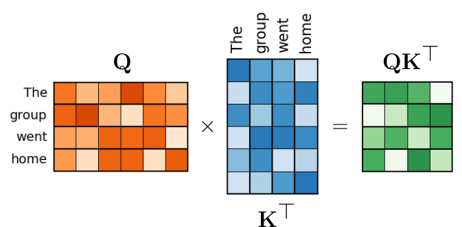
$\mathbf{Q}\mathbf{K}^\top$ now contains the attention scores for all pairs of words. The term "score" is commonly used to indicate that the values are, at least in principle, unbound since the dot product can range from $-\infty$ to $+\infty$.

Attention Weights

To ensure that the output vectors of the attention mechanism are of a similar magnitude, we need to normalize the (unbound) attention scores. More specifically we have to normalize $\mathbf{Q}\mathbf{K}^\top$ such that all values in a row sum up to $1$ — the reason for this will be clear in a bit. To accomplish this, we can simply apply the softmax function to $\mathbf{Q}\mathbf{K}^\top$ — to each row in $\mathbf{Q}\mathbf{K}^\top$ to be more precise. The figure below illustrates this operation using a $\mathbf{Q}\mathbf{K}^\top$ tensor with some arbitrary attention scores.

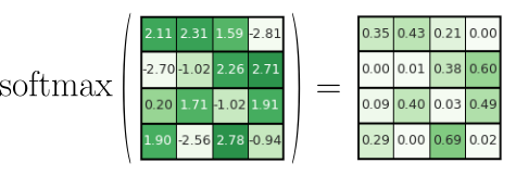
You can now check that in the output, all values within the same row sum up to $1$.

Attention Output

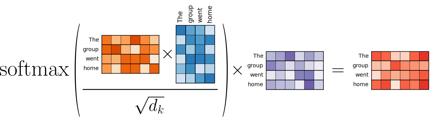
The last step of the attention mechanism is to calculate the output as the product of the attention weights and the value vectors in $\mathbf{V}$. This multiplication means that the output embedding of a word (e.g., "group") is calculated as the weighted sum of all the embedding vectors in $\mathbf{V}$, including the word itself. The figure below illustrates this operation:

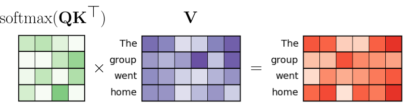
Notice here the importance of normalizing the rows in $\mathbf{Q}\mathbf{K}^\top$. Without it the values in the output vectors (red) may be of very different magnitudes compared to the value vectors (purple).

Putting Everything Together

Now that we went through the attention calculation step by step, we combine all steps into a single formula as shown below — this formula matches the notation in the original Transformer paper "Attention is all you Need".

$$\large \text{Attention}(\mathbf{Q}, \mathbf{K}, \mathbf{V}) = \text{softmax}\left(\frac{\mathbf{Q}\mathbf{K}^\top}{\sqrt{d_k}} \right) \mathbf{V} $$

Notice the one small extension in terms of the scaling factor $1/\sqrt{d_k}$ which we have not included in the step-by-step calculations above. This scaling factor is "only" important for computational reasons (and less for the concept of attention itself). It is used to prevent the dot products between query and key vectors from becoming too large as the dimensionality of the query, key, and value spaces increases. The purpose of this scaling is to stabilize the softmax operation. Without scaling, large dot products (which grow with $d_k$) could result in very large exponentials in the softmax, causing it to produce extremely small gradients — making training harder and potentially unstable. Dividing by $d_k$ keeps the values in a range where softmax can function effectively, leading to more stable gradients and better convergence during training. This is also why this specific attention calculation is called scaled dot-product attention. The figure below visualizes the the involved operations of the scaled dot-product attention.

Just to make the connection to the original Transformer paper "Attention is all you Need", the figure below is directly taken from that paper to describe the all involved operations to calculate the scaled dot-product attention.

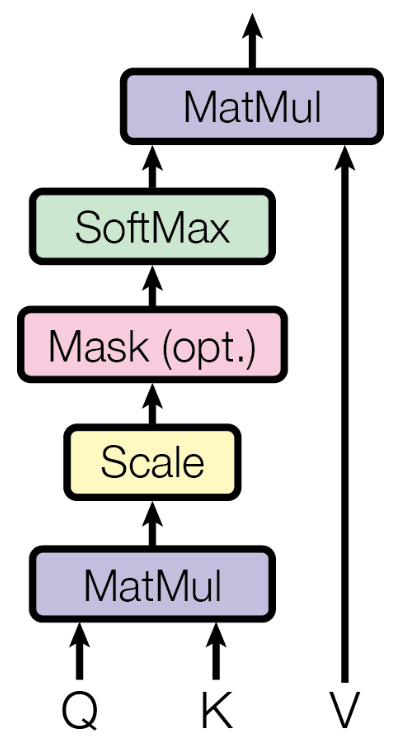
You will notice that optional operation of applying "Mask" to the scaled $\mathbf{Q}\mathbf{K}^\top$ tensor. The concept of masking is beyond the scope of this notebook and deserves its own detailed discussion.

In its core, scaled dot-product attention performs a very straightforward serions of matrix/tensor operations. As such, using libraries such as PyTorch that support the efficient execution of tensor/matrix operations, we can implement scaled dot-product attention with very few lines of code — again, we omit the idea of masking in this implementation — as shown in the code cell below:

class Attention(nn.Module):

    def __init__(self):
        super().__init__()

    def forward(self, Q, K, V):
        # Perform Q*K^T (* is the dot product here)
        out = torch.matmul(Q, K.transpose(1, 2))
        # Divide by square root scaling factor
        out = out / (K.shape[-1] ** 0.5)
        # Push throught softmax layer so that rows sum up to 1
        out = nn.functional.softmax(out, dim=-1)
        # Multiply with values V and return result
        return torch.matmul(out, V)

We run a working example once we have introduced the attention head. Notice that Attention assumes $\mathbf{Q}$, $\mathbf{K}$, $\mathbf{V}$ as input. It is the attention head that actually includes the transformation matrices $\mathbf{W}_q$, $\mathbf{W}_k$, and $\mathbf{W}_v$, that transform the input embeddings into the query, key, and values spaces. This also means that the Attention class itself does not contain any trainable parameters!

Self Attention vs. Cross Attention

The example we considered so far refers to the self-attention mechanism of in the encoder for Transformer-based machine translation setup — noticate that we only used the English input sentence "The group went home" so far. The encoder only utilized self-attention, although typically several self-attention blocks stacked on top of each other. This stacking is covered in more detail in the actual introduction of the full Transformer architectures — here, we focus on the core components of attention and multi-head attention.

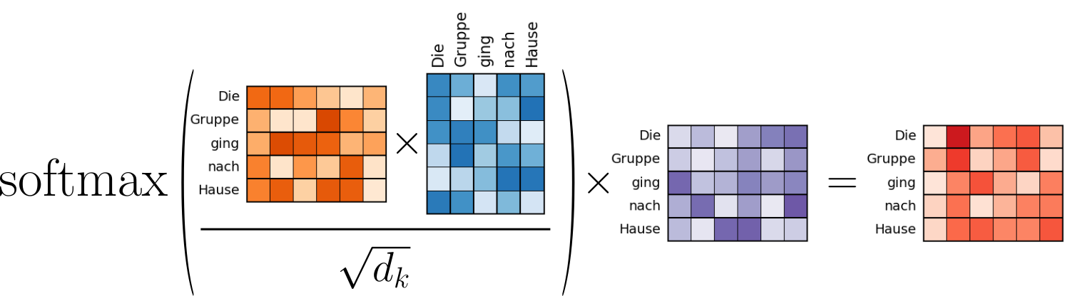
In contrast to the encoder, the decoder utilizes both the self-attention and cross attention. The self-attention in the decoder is completely analogous to the self-attention in the encoder, only that the input of the decoder is now the sequence in the target language (i.e., the German translation "The Gruppe ging nach Hause"). If we visualize the calculation of the self-attention for the decoder — see the figure below — you can clearly see how it matches the calculation of the self-attention in the encoder we have seen so far.

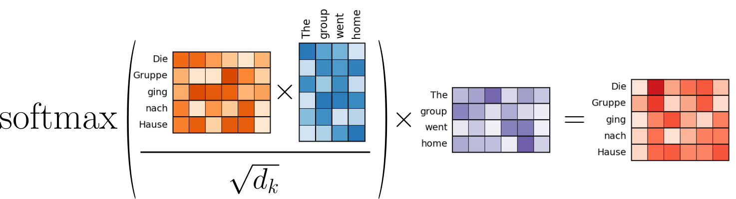
The purpose of cross attention is now to combine the encoder and decoder of the Transformer. After all, we want that the translation in the target language depends on the input sequence in the source language. Fundamentally, cross-attention still aims to recalculate the embedding vectors of the inputs words of our sequence "The Gruppe ging nach Hause". However, this recalculation should now depend on the output from the encoder. Recall that the output of the encoder is in essence simple the recalculated embedding vectors of the word in the sequence "The group went home".

In short, we still calculate the attention scores and attention weights based on two input sequences. The only difference is that two input sequences stem from different sources (i.e., the English and German input sentences). More specifically, the query vectors in $\mathbf{Q}$ derive from the embedding vectors for "The Gruppe ging nach Hause" (after the self-attention steps!), and both the key and value vectors in $\mathbf{K}$ and $\mathbf{V}$ derive from the output of the encoder — which, again, represent the recalculated embedding vectors of "The group went home" after the self-attention mechanism in the encoder. This, we can visualize the cross-attention operations in the decoder for our machine learning example as follows:

The notebook(s) covering to complete Transformer architecture provide more details on how attention is actually integrated in the encoder and decoder of the Transformer.

Attention Head

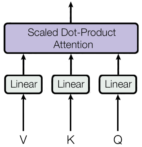
In the context of the Transformer architecture, the attention head represents the network component that combines the transformation of the input embeddings to the query, key, and value vectors — using the transformation matrices $\mathbf{W}_q$, $\mathbf{W}_k$, and $\mathbf{W}_v$ — with the scaled dot-product attention. The figure below is again adopted from the original Transformer paper "Attention is all you Need" representing an attention head:

Since we already implement the scaled dot-product attention in our Attention class, we can now implement the AttentionHead in a very straightforward manner. The class definition in the code cell below uses the variable name qkv_size to reflect that $d_q = d_k = d_v$. Apart from that, this class simply implements the transformation matrices as linear layers, as well as includes an instance of the Attention class.

class AttentionHead(nn.Module):
    
    def __init__(self, model_size, qkv_size):
        super().__init__()
        self.Wq = nn.Linear(model_size, qkv_size)
        self.Wk = nn.Linear(model_size, qkv_size)
        self.Wv = nn.Linear(model_size, qkv_size)
        self.attention = Attention()
        
    def forward(self, query, key, value):
        return self.attention(self.Wq(query), self.Wk(key), self.Wv(value))

To run an actual example, we can now create an instance of an attention head. To match out machine learning example, we need to set qkv_size = 6; the value for d_model we have already defined previously to match out example value of $d_{model} = 12$.

qkv_size = 6

encoder_self_attention_head = AttentionHead(d_model, qkv_size)
decoder_self_attention_head = AttentionHead(d_model, qkv_size)

Important: We need to create different instances of attention heads since each attention head comes with its own set of weight matrices. In simple terms, we cannot share the same attention head across the encoder and the decoder. After all, these two components serve different purposes.

Let's first consider self attention where the query, key, and values vectors all derive from the same input sequence — either the English sentence for the encoder, or the German sentence in the decoder. Since we do not care about the actual values here, the code below simply prints the shape of the output of the attention head instance.

encoder_self_attention_out = encoder_self_attention_head(input_en, input_en, input_en) # self-attention in encoder
decoder_self_attention_out = decoder_self_attention_head(input_de, input_en, input_en) # self-attention in decoder

print(f"Shape of output tensor for the encoder: {encoder_self_attention_out.shape}")
print(f"Shape of output tensor for the decoder: {decoder_self_attention_out.shape}")

Shape of output tensor for the encoder: torch.Size([1, 4, 6])
Shape of output tensor for the decoder: torch.Size([1, 5, 6])

As expected, the shape of the output is (batch_size, seq_len, qkv_size). Naturally, the sequence length seq_len depends on the size of the input sequence, which is $4$ for the encoder ("The group went home") and $5$ for the decoder ("Die Gruppe ging nach Hause").

We can now also create an attention head to handle the cross-attention in the decoder; the input parameters remain the same, of course.

decoder_cross_attention_head = AttentionHead(d_model, qkv_size)

We can now "mimic" the calculation of the cross-attention by using our example input embeddings. Keep in mind, however, that in practice the input for the cross attention are already recalculated embedding vectors. More specifically:

• input_de will be the recalculated embedding vectors for "The Gruppe ging nach Hause" after self-attention in the decoder

• input_de will be the recalculated embedding vectors for "The group went home" as the final output of the encoder

We will clarifies further down below once we introduce multi-head attention.

decoder_cross_attention_out = decoder_cross_attention_head(input_de, input_en, input_en)

print(f"Shape of output tensor for the decoder: {decoder_cross_attention_out.shape}")

Shape of output tensor for the decoder: torch.Size([1, 5, 6])

Of course, the shape of the output is again (batch_size, seq_len, qkv_size), with a sequence length of $5$ since we are in the decoder here.

Multi-Head Attention

So far, we only considered a single attention head, even if we used it for different purposes (self-attention and cross attention). However, the Transformer uses multiple attention heads to allow the model to focus on different types of relationships and patterns within the input sequence simultaneously. Each attention head operates independently, learning its own set of projections — that is the set of transformation matrices $\mathbf{W}_q$, $\mathbf{W}_k$, and $\mathbf{W}_v$ — for the queries, keys, and values. This means that one head might learn to focus on short-range syntactic dependencies (like subject-verb agreement), while another might capture long-range semantic relationships (like a pronoun referring back to a noun several tokens earlier).

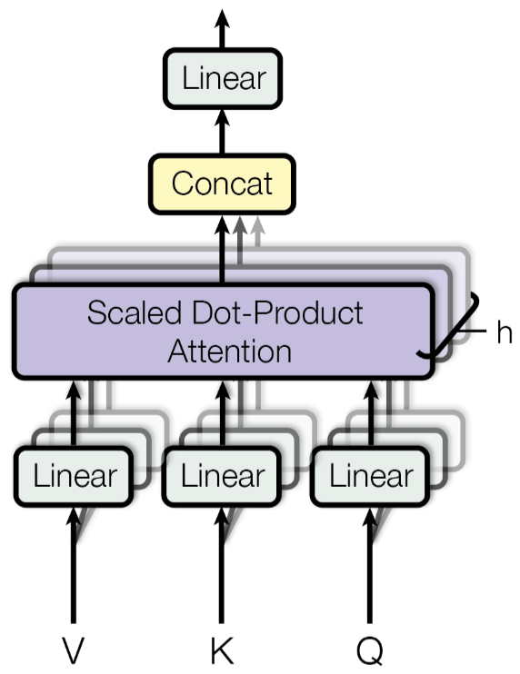
By using multiple heads, the Transformer can capture richer and more diverse contextual information than a single attention mechanism would allow. After each head computes its attention output, the results are concatenated and linearly transformed, combining insights from all heads into a unified representation. This multi-headed approach helps the model learn more nuanced representations of the input, which is especially useful in tasks like translation, summarization, or question answering, where understanding multiple layers of meaning is critical. The figure below from the Transformer paper shows the concept of multi-head attention. In this figure, $h$ represents the number of attention heads.

Using multiple heads makes the attention mechanism more expressive without significantly increasing the computational cost. Instead of using one large attention operation with high-dimensional vectors, the Transformer splits the work across multiple smaller heads, which are faster and easier to train in parallel. This design contributes to the model's effectiveness and scalability. The latter is realized by making the sizes of $d_k$ (recall that $d_q$ and $d_v$ have the same value) dependent on the embedding size $d_{model}$ and the number of heads $h$. More specifically,

$$\large d_k = d_{model} / h $$

where in practice $d_{model} \gg h$ and both values are chosen such that the result is an integer. For example, for our machine learning use case we already have $d_{model} = 12$. By assuming $h = 2$, we get $d_q = d_k = d_v = 6$ as we already used throughout the notebook. This relationship between $d_k$ and the number of heads $h$ ensures that the total number of trainable parameters — all trainable parameters in all weight matrices $\mathbf{W}_q$, $\mathbf{W}_k$, and $\mathbf{W}_v$ across all attention heads — remains the same when varying $h$. To show some numbers for real-world Transformer architectures, we can extend our previous table to include the number of heads and the results values for $d_k$:

Model	Architecture	$d_{model}$	$h$	$d_k$
BERT-base	encoder-only	768	12	64
BERT-large	encoder-only	1,024	16	64
GPT-3 Curie	decoder-only	2,048	32	64
GPT-3 Davinci	decoder-only	12,288	96	128
LLaMA 1/2/3 (7B)	decoder-only	4,096	32	128
LLaMA 1/2/3 (13B)	decoder-only	5,120	40	128
LLaMA 1/2/3 (70B)	decoder-only	8,192	64	128
T5-Base	encoder-decoder	768	12	64
T5-Large	encoder-decoder	1,024	16	64
BART-Base	encoder-decoder	768	12	64
BART-Large	encoder-decoder	1,024	16	64

Despite multiple attention heads, and with each individual attention head producing its own output, the final output of the multi-head attention layer is still one recalculated embedding vector for each word in the original input sequences. In fact, the size of the final output embeddings are the same as the size of the input embeddings (e.g., $d_{model}=12$ in our example). This allows that in the Transformer architecture multiple blocks containing several multi-head attention layers can easily be stacked above each other.

To accomplish this, the output of all attention heads in the same multi-head attention layer are first concatenated into a single tensor. Since $d_k = d_{model} / h$, the embedding vectors in these concatenated tensors have again a size of $d_{model}$. However, this tensor does not form the final output, instead this tensor is multiplied by another weight matrix $\mathbf{W}_o$. For one, this adds additional trainable parameters to the layer and therefore additional capacity for the Transformer model to learn. And also, this output weight matrix makes the multi-head attention layer more flexible in case the values of $d_q$, $d_k$, and $d_v$ are not always identical and do not derive from $d_{model} / h$ — in which case the embeddings in the concatenated tensor not necessary of size $d_{model}$ anymore. However, in the basic Transformer architecture, the output weight matrix $\mathbf{W}_o$ is defined as:

$$\large \mathbf{W}_o \in \mathbb{R}^{d_{model}\times d_{model}} $$

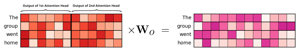
The figure below shows the concatenation step and the matrix multiplication operation with $\mathbf{W}_o$ for our example machine translation user case with $d_{model} = 12$ and $h=2$ and therefore $d_q = d_k = d_v = 6$:

Note that we could have also set $h=3$ or $h=4$, in which case the size of the query, key, and value vectors be $d_q = d_k = d_v = 4$ or $d_q = d_k = d_v = 6$. But no matter the value of $h$, the total number of trainable parameters — captured by the weight matrices $\mathbf{W}_q$, $\mathbf{W}_k$, and $\mathbf{W}_v$ in each individual attention head together with the output weight matrix $\mathbf{W}_o$ — will remain the same.

Lastly, let's look at a very basic implementation of multi-head attention. Since we already have our AttentionHead class, this is a straightforward task. The input parameters for the constructor of MultiHeadAttention is model_size (representing $d_{model}$) and num_heads (representing $h$). From this, we can first derive qkv_size (representing the value for $d_q = d_k = d_v$). The main attributes of the class are the list of attention heads — implemented as a list of instances of the class AttentionHead — and the output weight matrix Wo (representing $W_o$). The forward() method performs all the operations we have just covered: concatenating the outputs of all attention heads and projecting them into the output space.

class MultiHeadAttention(nn.Module):
    
    def __init__(self, d_model, num_heads):
        super().__init__()
        # Define sizes of Q/K/V based on model size and number of heads
        self.qkv_size = d_model // num_heads
        #        
        self.heads = nn.ModuleList(
            [AttentionHead(d_model, self.qkv_size) for _ in range(num_heads)]
        )
        # Linear layer to "unify" all heads into one
        self.Wo = nn.Linear(d_model, d_model)
        
    def forward(self, query, key, value):
        # Push Q, K, V through all the Attention Heads
        out_heads = tuple([ attention_head(query, key, value) for attention_head in self.heads ])
        # Concatenate the outputs of all Attention Heads
        out = torch.cat(out_heads, dim=-1)
        # Push concatenated outputs through last layers and return result
        return self.Wo(out)

Keep in mind that this implementation assumes that the values for d_model and num_heads are choses such that d_model // num_heads has no remainder. In practice, this should be checked and an exception should be raised if there is a remainder.

Like before, we can create instances of MultiHeadAttention to test the implementation. Let's start with the multi-head attention layers for the self-attention in the encoder and the decoder. Feel free to set num_heads to other meaningful values — proper factors of 12 such as 3, 4, or 6. This should not affect the final output put shape of the multi-head attention layer.

num_heads = 2

encoder_self_mha = MultiHeadAttention(d_model, num_heads)
decoder_self_mha = MultiHeadAttention(d_model, num_heads)

We can now give both instances their respective inputs, that is, the English sequence to the encoder and the German sequence to the decoder.

encoder_self_mha_out = encoder_self_mha(input_en, input_en, input_en)
decoder_self_mha_out = encoder_self_mha(input_de, input_de, input_de)

print(encoder_self_mha_out.shape)
print(decoder_self_mha_out.shape)

torch.Size([1, 4, 12])
torch.Size([1, 5, 12])

Now we can see that the size of the output embedding vectors is indeed the same as the size of the input embedding vectors. This means we could feed this output as input into another multi-head attention layer. For the decoder, this includes that we can now use the output of the decoder self-attention layer as input for the decoder cross-attention layer. For this, let's first create this layer as another instance of MultiHeadAttention.

decoder_cross_mha = MultiHeadAttention(d_model, num_heads)

The code cell below calculates the cross-attention. Recall that here the query vectors derive from the output of the decoder self-attention layer. In contrast, both the key and value vectors derive from the output of the encoder.

decoder_cross_mha_out = decoder_cross_mha(decoder_self_mha_out, encoder_self_mha_out, encoder_self_mha_out)

print(decoder_cross_mha_out.shape)

torch.Size([1, 5, 12])

Important: In the full Transformer architecture, the output of one multi-head attention layer is not directly passed into another multi-head attention layer but first passed through other components. Those code snippets merely illustrate the relationship between the different self-attention and cross-attention layers.

---

Discussion — What's Next?

The concepts of attention and multi-head attention arguably form the backbone of the Transformer architecture. In this notebook, we first explored the fundamental intuition behind attention and covered in detail all involved operations and calculations. With this solid understanding of attention and multi-head attention, you are now equipped to delve into the complete Transformer architecture and its practical implementations. Here are some concrete follow-up considerations.

Masking

We already briefly discussed that Attention class implementing the scaled dot-product attention is missing the so-called masking step. While not fundamental to the concept of attention, masking is often required when training Transformer-based models practice. In a nutshell, masking in the Transformer architecture serves to control which parts of the input sequence a word is allowed to attend to during the attention mechanism. It modifies the attention weights by setting certain positions to negative infinity, effectively nullifying their influence in the softmax computation — since $-\infty$ becomes $0$ after softmax. This is crucial for maintaining the integrity of the model's structure and learning objectives. There are two main types of masking commonly used in Transformers:

• Padding Mask: This type of mask ensures that the model does not attend to padding tokens, which are inserted to make all input sequences in a batch the same length. Since padding carries no meaningful information, attending to it would waste computation and could negatively impact model learning. Padding masks are typically used in both the encoder and decoder.

• Causal (or Look-Ahead) Mask: This mask is used in the decoder during training to prevent a position from attending to future positions in the sequence. For example, when predicting the next word in a sentence, the model should not have access to words that come later in the sequence. The causal mask enforces this autoregressive property by masking out all future positions.

Overall, masking ensures that the attention mechanism behaves appropriately depending on the context — whether that means ignoring irrelevant padding tokens or preserving the autoregressive nature of sequence generation. It's a subtle but critical detail that allows the Transformer to function correctly and efficiently across different tasks. Giving its importance, we therefore cover masking as its own topic in full detail.

Towards the Full Transformer Architecture

While asking is an extension to the implementation of the scaled dot-product attention, the complete Transformer architecture features more components and operations beyond the multi-head attention layers. The figures below is taken from the original Transformer paper "Attention is all you Need" shows the complete architecture with the encoder and decoder, and highlights the parts which we covered in this notebook — the multi-head attention layers.

The figure above makes it clear that apart from the multi-head attention layers, the Transformer architecture consists of several other crucial components that contribute to its performance and flexibility. To give a brief overview here, some of these important components include:

• Positional Encoding. Since the Transformer does not inherently understand the order of tokens due to its non-recurrent architecture, positional encoding is introduced to inject information about the relative or absolute position of each token in the sequence. This is done by adding a positional vector to each token embedding. These vectors can be fixed (using sinusoidal functions) or learned during training. The inclusion of positional encoding ensures that the model can differentiate between sequences like "dog bites man" and "man bites dog". It enables the attention mechanisms to take token positions into account when computing contextual relationships, preserving the sequential structure necessary for understanding natural language.

• Feedforward Neural Network (FFN). Each layer in both the encoder and decoder contains a feedforward neural network that operates independently on each position in the sequence. This component typically consists of two linear transformations with a non-linear activation function in between. The first linear layer expands the dimensionality, while the second reduces it back to the original model size $d_{model}$. The FFN acts as a powerful local transformation, allowing the model to process and refine information for each token position without interference from others. This helps the model capture more abstract features that attention alone might not be able to represent.

• Layer Normalization. Layer normalization is applied within each sublayer of the Transformer (i.e., after the attention mechanism and the feedforward network). It normalizes the inputs across the feature dimension for each token, helping to stabilize and accelerate training by reducing internal covariate shift. This is especially important in deep architectures, where the distribution of inputs can change significantly from one layer to the next. By standardizing the scale and distribution of activations, layer normalization enables smoother gradient flow and often leads to faster convergence. It works in conjunction with residual connections to ensure that learning remains stable and that deep networks can be trained more effectively.

• Residual Connections. Residual (or skip) connections are used around each sublayer (attention and feedforward) to allow the model to retain the original input and add the transformation on top of it. This technique helps mitigate the vanishing gradient problem and allows gradients to flow more easily through deeper networks. The idea behind residual connections is that it's easier to learn a small adjustment to the identity function than to learn the full transformation from scratch. This not only helps with optimization but also encourages feature reuse, improving model performance and convergence speed.

• Encoder and Decoder Stacks. The Transformer is structured around stacked layers of encoders and decoders. Each encoder layer includes a self-attention sublayer followed by a feedforward network, while each decoder layer includes an additional encoder-decoder attention sublayer that allows it to attend to encoder outputs. These stacks enable the model to build deep and complex representations of both input and output sequences.

Again, while attention is at the heart of the Transformer architecture, it is a combination of multiple components and concepts that make Transformers show state-of-the-art performances for real-world tasks. These components and the overall Transformer architecture are covered in more detail in other notebooks.

Optimization

In this notebook, we provide basic implementations for the scaled dot-product attention, attention heads, as well as multi-head attention layers to make the operations underlying the attention mechanisms and extensions more tangible. However, all code examples focus on simplicity and readability without performance considerations. For example, notice that the AttentionHead class implements three linear layers (nn.Linear) representing the three projection matrices $W_q$, $W_k$, and $W_v$. In practice these there linear layers are often implemented using a single linear layer, say, $\mathbf{W}_a$ ("a" for attention) with $\mathbf{W}_a \in \mathbb{R}^{d_{model}\times d_k}$. Using this approach, the query, key, and value vectors can then be retrieved by splitting the output tensor after the projection using $W_a$. This approach generally shows a better performance in terms of training and inference time. While the changes to the code are small, using three separate linear layers are more intuitive to comprehend.

Another issue in terms of performance is the quadratic runtime of the attention mechanisms. For example, in case of self-attention and assuming an input sequence of length $N$, we need to calculate $N^2$ attention scores and attention weights. While the input sequences for our toy example were very short (only 4 and 5 words), in practice, the input sequences can be very long, potentially containing many hundreds or thousands of words. This becomes a major bottleneck when dealing with long sequences, leading to high memory usage and slow computation, which limits the scalability of standard Transformers. To address this, different strategies to improve performance have been proposed, e.g.:

• Sparse Attention: Instead of attending to all tokens, the model attends only to a subset (e.g., local neighborhoods or pre-defined patterns). Examples include Longformer, BigBird, and Sparse Transformers, which reduces complexity by imposing sparse attention structures.

• Low-Rank Approximations: Techniques like Linformer and Performer approximate the full attention matrix using low-rank projections or kernel methods, reducing complexity to linear or near-linear time while preserving performance.

• Memory Compression: Models like Reformer use locality-sensitive hashing to group similar tokens and compute attention only within those groups, cutting down on redundant computations.

• Hierarchical or Chunking Approaches: These divide long sequences into smaller segments (chunks) and process them individually before combining the outputs, sometimes using additional global tokens to retain context across chunks.

These strategies aim to make Transformers more scalable while maintaining or improving training and inference time, enabling their application to domains that require processing long sequences efficiently. On the other hand, such strategie may lead to some loss of information as part of the attention mechanism and may (slightly) degrade its effectiveness. However, minor degradation in effectiveness are often accepted in practice in exchange for noticeable improvements in efficiency, particularly very large models such as foundational Large Language Models (LLMs).

---

Summary

To sum up, attention is a mechanism that allows models to focus on the most relevant parts of an input sequence when generating an output. Instead of treating all input elements equally, attention assigns different weights to different parts, enabling the model to selectively process information based on its importance to the task at hand. This approach has revolutionized natural language processing (NLP), allowing for more effective handling of long-range dependencies within text sequences.

Multi-head attention extends the basic attention mechanism by running multiple attention operations, or "heads", in parallel. Each head learns to focus on different aspects of the input, capturing diverse patterns and relationships. The outputs of all heads are then concatenated and linearly transformed, providing the model with a richer and more nuanced representation of the input. This diversity is crucial for capturing complex linguistic features such as syntax, semantics, and word order.

In the Transformer architecture, attention — specifically scaled dot-product attention and multi-head attention — is the core building block. Transformers forgo recurrence entirely and rely on self-attention mechanisms to process sequences in parallel. This design not only speeds up training but also improves the ability to model long-range dependencies more efficiently than earlier models like RNNs and LSTMs. Attention and multi-head attention are fundamental to the success of Transformers in a wide range of tasks. Their ability to dynamically prioritize relevant information has enabled unprecedented advances in performance and generalization across many domains.