Disclaimer: This Jupyter Notebook contains content generated with the assistance of AI. While every effort has been made to review and validate the outputs, users should independently verify critical information before relying on it. The SELENE notebook repository is constantly evolving. We recommend downloading or pulling the latest version of this notebook from Github.
Backpropagation
Backpropagation, short for "backward propagation of errors," is a foundational algorithm in the field of machine learning and artificial intelligence. At its core, it is a method used to train artificial neural networks by efficiently computing gradients that guide the optimization of the network's parameters. Introduced in the 1980s, backpropagation became a breakthrough that catalyzed the rapid growth of neural networks and deep learning, which are now central to modern AI applications like natural language processing, image recognition, and recommendation systems.
The importance of backpropagation lies in its ability to adjust the weights and biases of a neural network to minimize errors in predictions. It works by propagating the error, computed at the output layer, backward through the network to update each layer's parameters. This process leverages the chain rule of calculus to compute how changes in the parameters of the network influence the output. By iteratively applying backpropagation during training, the network learns to approximate complex, non-linear relationships within the data.
Learning about backpropagation is crucial because it forms the backbone of how neural networks learn and generalize. Understanding this algorithm allows practitioners to appreciate the inner workings of models they use, diagnose issues such as vanishing or exploding gradients, and make informed decisions about architecture design or hyperparameter tuning. Moreover, concepts derived from backpropagation underpin other advanced techniques, such as transfer learning and fine-tuning pre-trained models.
From a broader perspective, backpropagation exemplifies the synergy between mathematics and computer science in solving real-world problems. It highlights how mathematical principles can be translated into computational algorithms with transformative societal impacts. For anyone entering the field of AI or deep learning, grasping backpropagation is a foundational step toward mastering the broader landscape of machine learning techniques.
Preliminaries
Basic Notations
y denotes the output of a function $f$ that takes one or more parameters as input, and applies various operations (e.g., addition, multiplication, squaring, logarithm, etc.) to calculate an output.
$x_1$, $x_2$, $x_3$,... denote input parameters of a multivariable function $f$
$u_1$, $u_2$, $u_3$, ... denote intermediate results based on a subset of operations in $f$
Quick Recap: Chain Rule
Many parametric machine learning models — most prominently neural networks — are trained through minimizing a loss function using gradient-based methods. Here, the model and its performance is determined by the current set of parameters (or weights) $\mathbf{w}$. The loss function quantifies this performance, and minimizing the loss function means finding the weights $\mathbf{w}$ where the model performs best. Gradient-based methods calculate the gradient of the loss function with respect to all weights $\mathbf{w}$ to then systematically change the weights to decrease the loss.
Calculating the gradient requires calculating the derivative of a function — or all partial derivatives of a multivariable function. In case more complex models such a neural networks, calculating the derivative and therefore the gradient can be quite challenging. The chain rule is essential in calculus because it allows us to differentiate complex functions by breaking them into simpler components. It is widely used in various fields, including physics, engineering, and economics. In machine learning, the chain rule is the mathematical foundation of backpropagation, enabling the computation of gradients for training neural networks.
The chain rule in calculus provides a way to compute the derivative of a composite function. Suppose $y$ depends on $u$, and $u$ in turn depends on $x$, i.e., $y=f(u)$ and $u=g(x)$. The chain rule states that the derivative of $y$ with respect to $x$ can be found by multiplying the derivative of $y$ with respect to $u$ by the derivative of $u$ with respect to $x$.
$$\large \frac{d y}{d x} = \frac{d y}{d u} \cdot \frac{d u}{d x} $$Here:
- $\large \frac{dy}{dx}$ is the rate of change of $y$ with respect to $x$,
- $\large \frac{dy}{du}$ is the rate of change of $y$ with respect to $u$,
- $\large \frac{du}{dx}$ is the rate of change of $u$ with respect to $x$.
To give a very simple example, consider the function $y = f(x) = sin(x^2)$. As a composite function, we can define $y = sin(u)$ and $u = x^2$. To find $\large \frac{d y}{d x}$, we use the chain rule as follows
Calculate $\large \frac{du}{dx}$: $$\large \frac{du}{dx} = 2x$$
Calculate $\large \frac{dy}{du}$: $$\large \frac{dy}{du} = cos(u)$$
Calculate $\large \frac{dy}{dx}$ by using the chain rule: $$\large \frac{d y}{d x} = \frac{d y}{d u} \cdot \frac{d u}{d x} = cos(u)\cdot 2x$$
Substitute $u=x^2$: $$\large \frac{d y}{d x} = cos(x^2)\cdot 2x$$
The chain rule is crucial for training neural networks because it enables efficient computation of gradients during backpropagation. These gradients indicate how to adjust weights and biases to minimize prediction errors. By applying the chain rule layer by layer, optimization methods like gradient descent can update parameters effectively, making training deep networks feasible. How backpropagation works in detail using examples is the topic of this notebook.
Computational Graphs
A computational graph is a visual representation used in machine learning and deep learning to depict the sequence of operations performed on data as it moves through a computational process, particularly during forward and backward propagation. Each node in the graph represents a variable or operation (e.g., addition, multiplication, or activation functions), and the edges represent the flow of data between these nodes. The computational graph is a common visualization tool because it provides a clear and intuitive understanding of complex computations. It highlights the dependencies between variables and operations, making debugging and optimization easier. Moreover, modern frameworks like TensorFlow and PyTorch utilize computational graphs internally to manage and optimize the execution of machine learning models, reinforcing their importance as a fundamental concept in deep learning workflows.
To give an example, the figure below shows the computational graph for the function $y = f(x) = sin(x^2)$ from above. The first node in the graph represents the squaring operation $u = x^2$; the second node represents the calculation $sin(u)$.
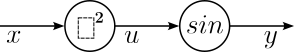
This representation of a composite function using a computation graph is very useful for understanding the underlying concepts of backpropagation.
Backpropagation Explained by Examples
Simple Example
Let's start with a very simple example and consider the following multivariable function:
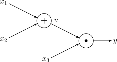
$$\large y = f(x_1, x_2, x_3) = (x_1 + x_2)x_3 $$We can define the addition and multiplication operations as their own functions: $u = x_1 + x_2$ and $y = ux_3$. Considering these two operations as nodes, the corresponding computational graph looks as follows:
Given this graph, we can already write down the equations for calculating the local gradients for all computational nodes:
Node |
Local Gradients |
|---|---|
| $$\large u = x_1 + x_2$$ | $$\large \frac{\partial u}{\partial x_1} = 1\ , \quad \frac{\partial u}{\partial x_2} = 1 $$ |
| $$\large y = u x_3$$ | $$\large \frac{\partial y}{\partial u} = x_3\ , \quad \frac{\partial y}{\partial x_3} = u$$ |
Forward Pass
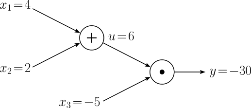
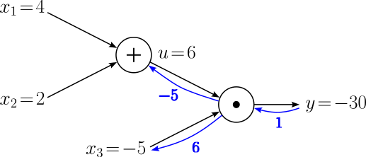
The forward pass is the process of evaluating the mathematical expression represented by computational graphs. Doing the forward pass means passing the values from all inputs in the "forward" direction from the left (input) to the right where the output is. For our example here, let's assume the input values $x_1 = 4$, $x_2 = 2$, and $x_3 = -5$. With that, we can easily calculate the values of $u$ and $y$ and visualize all values in our computational graph:
Backward Pass
In the backward pass, the goal is now to compute the gradients for each input $x_i$ with respect to the final output $y$. When training neural networks, the inputs of nodes in the computational graphs will include all trainable weights $\mathbf{w}$, so we need their gradients to update the weights when using methods such as Gradient Descent. For our example, we need to calculate the following gradients:
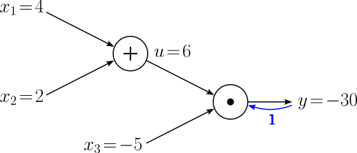
$$ \large \frac{\partial y}{\partial x_1},\ \large \frac{\partial y}{\partial x_2},\ \large \frac{\partial y}{\partial x_3} $$The fundamental idea of backpropagation is to calculate all derivatives from the output to the input following the respective path in the computational graph. for example, backpropagation calculates the gradient of $\large \frac{\partial y}{\partial x_1}$ by calculating the following partial derivatives using the chain rule:
$$ \large \frac{\partial y}{\partial y} \longrightarrow \frac{\partial y}{\partial u} \longrightarrow \frac{\partial y}{\partial x_1} $$The first partial derivative $\large \frac{\partial y}{\partial y}$, i.e., the partial derivative of the output with respect to the output, seems a bit pointless, but we will see later how it fits the systematic process and backpropagation. Trivially, the gradient for any output value $y$ is $\large \frac{\partial y}{\partial y} = 1$. And we can add this information about our first gradient into our computational graph.
Passing backward through the computational node for the multiplication operation means calculating the gradients with respect to the $u$ and $x_3$. For this, we can apply the chain rule accordingly:
$$ \begin{align} \large \frac{\partial y}{\partial u} &= \large \frac{\partial y}{\partial y}\cdot \frac{\partial y}{\partial x_3} \\[0.5em] \large \frac{\partial y}{\partial x_3} &= \large \frac{\partial y}{\partial y}\cdot u \\[0.5em] \end{align} $$Again, having $\large \frac{\partial y}{\partial y}$ seems not really required. However, notice that we calculate both gradients by multiplying the gradient coming in from the output of the computational node — which we calculated in the previous step — and the local gradient of the corresponding input node. Furthermore, we also know the local gradients, either because it is an input variable (here $x_3$) or an intermediate result we calculated during the forward pass (here $u$). In other words, while we could calculate $u = x_1 + x+2$ again, it is much more efficient to save the result during the forward pass and re-use it for the backward pass. Plugging all values gives us the following gradients:
$$ \begin{align} \large \frac{\partial y}{\partial u} &= \large \frac{\partial y}{\partial y}\cdot \frac{\partial y}{\partial u} = 1\cdot x_3 = -5 \\[0.5em] \large \frac{\partial y}{\partial x_3} &= \large \frac{\partial y}{\partial y}\cdot u = 1\cdot 6 = 6\\[0.5em] \end{align} $$Let's add these gradients to our computational graph.
The computational node the backpropagate through is the one for the addition operation to calculate the gradients of the output with respect to $x_1$ and $x_2$. The process is exactly the same as we just have seen of the multiplication operation. Using the chain rule, we can write:
$$ \begin{align} \large \frac{\partial y}{\partial x_2} &= \large \frac{\partial y}{\partial u}\cdot \frac{\partial u}{\partial x_2} \\[0.5em] \large \frac{\partial y}{\partial x_1} &= \large \frac{\partial y}{\partial u}\cdot \frac{\partial u}{\partial x_1} \\[0.5em] \end{align} $$The shared factor $\large \frac{\partial y}{\partial u} = -5$ is again the gradient coming in from the output of the computational node we have just calculated. Similarly, the factors $\large \frac{\partial u}{\partial x_2}$ $\large \frac{\partial u}{\partial x_1}$ are the local gradients of the inputs of the node. We can therefore calculate the last two remaining gradients with respect to the inputs $x_2$ and $x_1$:
$$ \begin{align} \large \frac{\partial y}{\partial x_2} &= \large -5\cdot 1 = -5 \\[0.5em] \large \frac{\partial y}{\partial x_1} &= \large -5\cdot 1 = -5\\[0.5em] \end{align} $$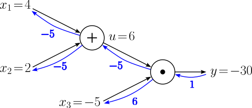
We have now calculated all gradients $\large \frac{\partial y}{\partial x_1}$, $\large \frac{\partial y}{\partial x_2}$, and $\large \frac{\partial y}{\partial x_3}$ using backpropagation. Despite this very simple example, we saw the core aspects of backpropagation: (a) the application of the chain rule, and (b) the re-use of the intermediate results calculated during the forward pass.
Advanced Example
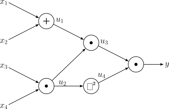
For some additional practice, let's extend our initial multivariable function by additional inputs as well as operations. While this does not require any additional step we have not seen before, a more complex function better highlights the benefits of systematically calculating all gradients step by step. In this more advance example, we will work with the following function:
$$\large y = f(x_1, x_2, x_3, x_4, x_5) = (x_1 + x_2)x_3\cdot (x_4x_5)^2 $$The first step is, again, to split this composite function into meaningful operation. Given that the function is still rather simple, we treat each addition, multiplication, and squaring operation as their own node in the computational graph. This gives us the computational graph as shown below.
As we need this information later for the backward pass of the backpropagation procedure, let's list all local gradients for each computational node.
Node |
Local Gradients |
|---|---|
| $$\large u_1 = x_1 + x_2$$ | $$\large \frac{\partial u_1}{\partial x_1} = 1\ , \quad \frac{\partial u_1}{\partial x_2} = 1 $$ |
| $$\large u_2 = x_3x_4$$ | $$\large \frac{\partial u_2}{\partial x_3} = x_4\ , \quad \frac{\partial u_2}{\partial x_4} = x_3$$ |
| $$\large u_3 = u_1 u_2$$ | $$\large \frac{\partial u_3}{\partial u_1} = u_2\ , \quad \frac{\partial u_3}{\partial u_2} = u_1$$ |
| $$\large u_4 = u_2^2$$ | $$\large \frac{\partial u_4}{\partial u_2} = 2u_2$$ |
| $$\large y = u_3u_4$$ | $$\large \frac{\partial y}{\partial u_3} = u_4\ , \quad \frac{\partial y}{\partial u_4} = u_3$$ |
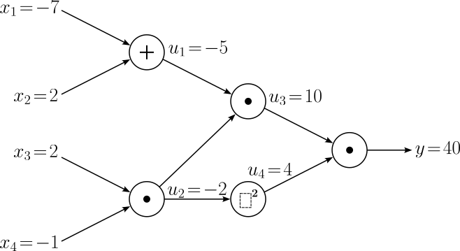
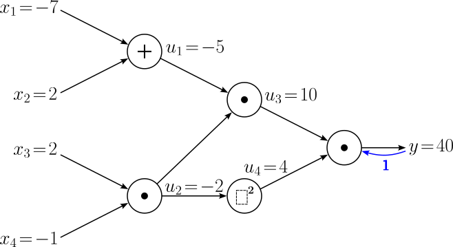
Forward Pass
The forward pass is straightforward as usually as we simply calculate the final output $y$ as well as all intermediate results $u_i$ as given by the computational graph. We assume that the values for our five input variables are $x_1 = -7$, $x_2 = 2$, $x_3 = 2$, and $x_4 = -1$. The computational below now includes all input values $x_i$, intermediate results $u_i$, and the final output value $y$.
Backward Pass
With five inputs, we now need to calculate the gradients of the function with respect to all five input variables. More specifically, we are looking for
$$ \large \frac{\partial y}{\partial x_1},\ \large \frac{\partial y}{\partial x_2},\ \large \frac{\partial y}{\partial x_3},\ \large \frac{\partial y}{\partial x_4} $$Now that the function and therefore the computational graph is a bit more complex, the path from the output to the inputs has also become a bit longer. This means that we have to compute more intermediate gradients. The example below illustrate all the gradients backpropagation will calculate to finally be able to calculate the gradient for $\large \frac{\partial y}{\partial x_1}$:
$$ \large \frac{\partial y}{\partial y} \longrightarrow \frac{\partial y}{\partial u_3} \longrightarrow \frac{\partial y}{\partial u_1} \longrightarrow \frac{\partial y}{\partial x_1} $$As usual, we begin with our "trivial" gradient $\large \frac{\partial y}{\partial y} = 1$. Again, we explicitly include this gradient to adhere to our procedure by calculating all following gradients for each computational node by multiplying the incoming gradient from the output with the corresponding in local gradients. Let's add this "trivial" gradient to our computational graph.
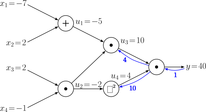
Now the "real" backpropagation starts by considering the first computation node (with respect to the backward pass). Passing backward through the computational node for the multiplication operation means calculating the gradients with respect to the $u$ and $x_3$. For this, we can apply the chain rule accordingly:
$$ \begin{align} \large \frac{\partial y}{\partial u_3} &= \large \frac{\partial y}{\partial y}\cdot \frac{\partial y}{\partial u_3} \\[0.5em] \large \frac{\partial y}{\partial u_4} &= \large \frac{\partial y}{\partial y}\cdot \frac{\partial y}{\partial u_4} \\[0.5em] \end{align} $$Backpropagation ensures that we always have both factors on the right-hand side of the equations. Firstly, $\large \frac{\partial y}{\partial y}$ we have just calculated on the previous step. And secondly, both gradients $\large \frac{\partial y}{\partial u_3}$ and $\large \frac{\partial y}{\partial u_4}$ are known since they are they reflect intermediate results calculated during the forward pass, here $u_4$ and $u_3$. By plugging in those values we get:
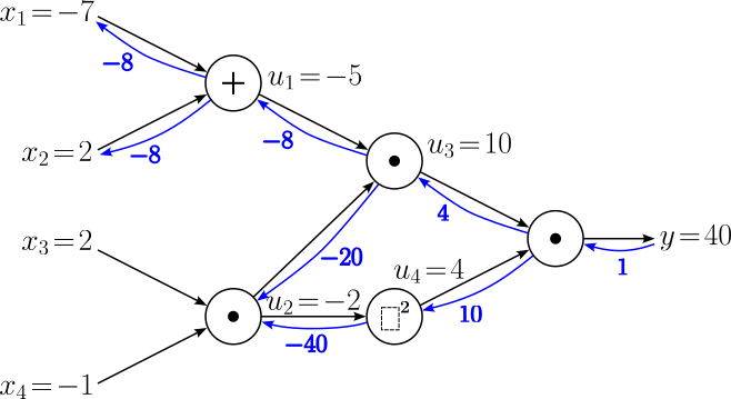
$$ \begin{align} \large \frac{\partial y}{\partial u_3} &= \large 1\cdot u_4 = \large 1\cdot 4 = 4 \\[0.5em] \large \frac{\partial y}{\partial u_4} &= \large 1\cdot u_3 = \large 1\cdot 10 = 10\\[0.5em] \end{align} $$Let's add these gradients also to our computational graph.
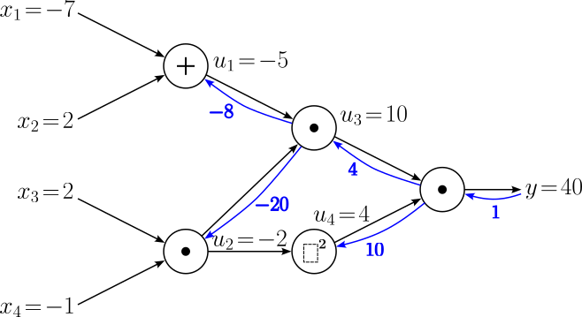
Now the process gets a bit more interesting compared to the simple example as we have two separate operations (i.e., computational nodes) we need to backpropagate through. However, this does not change anything in the process itself, we only have to handle each operation individually to calculate all gradients. So let's start with the multiplication operation that gives us the intermediate result $u_3 = 10$. This means we are interested in the gradients $\large \frac{\partial y}{\partial u_1}$ and $\large \frac{\partial y}{\partial u_2}$. However, you might have noticed that node $u_2$ feeds into more than one other node — or simply speaking, the node yielding $u_2$ has two outgoing edges. This means there are two different paths going from that node to the output $y$. When backpropagating through the multiplication node $u_3$ we only cover one path for the time being. Let's annotate this explicitly when applying the chain rule: $$ \begin{align} \large \frac{\partial y}{\partial u_1} &= \large \frac{\partial y}{\partial u_3}\cdot \frac{\partial u_3}{\partial u_1} \\[0.5em] \large \frac{\partial y^{[1]}}{\partial u_2} &= \large \frac{\partial y}{\partial u_3}\cdot \frac{\partial u_3}{\partial u_2} \\[0.5em] \end{align} $$
We just calculated $\large \frac{\partial y}{\partial u_3} = 4$, and we already know the local gradients $\large \frac{\partial u_3}{\partial u_1} = u_2$ and $\large \frac{\partial u_3}{\partial u_2} = u_1$. Together with the intermediate results calculated during the forward pass, we get:
$$ \begin{align} \large \frac{\partial y}{\partial u_1} &= \large 4\cdot u_2 = 4\cdot (-2) = -8 \\[0.5em] \large \frac{\partial y^{[1]}}{\partial u_2} &= \large 4\cdot u_1 = 4\cdot (-5) = -20\\[0.5em] \end{align} $$So we have two more gradients we can add to our computational graph.
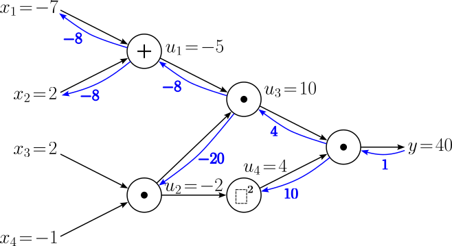
For the next step, we can consider either the addition operation that resulted in $u_1 = -5$ or the squaring operation that resulted in $u_4 = 4$. Let's go with the former, meaning we want to calculated the gradients $\large \frac{\partial y}{\partial x_1}$ and $\large \frac{\partial y}{\partial x_2}$, two of the five gradients of the input variables. The chain rules tells us that we can calculate both gradients as:
$$ \begin{align} \large \frac{\partial y}{\partial x_1} &= \large \frac{\partial y}{\partial u_1}\cdot \frac{\partial u_1}{\partial x_1} \\[0.5em] \large \frac{\partial y}{\partial x_2} &= \large \frac{\partial y}{\partial u_1}\cdot \frac{\partial u_1}{\partial x_2} \\[0.5em] \end{align} $$With $\large \frac{\partial y}{\partial u_1} = -8$ and the two local gradients we already know, $\large \frac{\partial y}{\partial x_1}$ and $\large \frac{\partial y}{\partial x_2}$ evaluate to:
$$ \begin{align} \large \frac{\partial y}{\partial x_1} &= \large -8\cdot 1 = -8 \\[0.5em] \large \frac{\partial y}{\partial x_2} &= \large -8\cdot 1 = -8 \\[0.5em] \end{align} $$Another two gradients to be added to our computational graph. We are almost there.
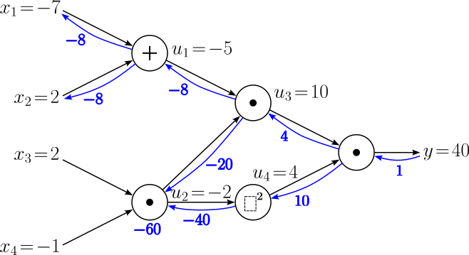
The next computational node we have to backpropagate through is the squaring operations that gave us $u_4 = 4$, which will again(!) give us the gradient for $\large \frac{\partial y}{\partial u_2}$. Notice how we now reached node $u_2$ using the second path. Applying the chain rule — and adding the explicit annotation again — we can calculate this gradient using known information:
$$ \begin{align} \large \frac{\partial y^{[2]}}{\partial u_2} &= \large \frac{\partial y}{\partial u_4}\cdot \frac{\partial u_4}{\partial u_2} \\[0.5em] \end{align} $$Note that here we calculate a single new gradient as the squaring a number is an unary operation. Recall that we have calculated $\large \frac{\partial y}{\partial u_4} = 10$ several steps before; see above. And as usual, we also have the value of required local gradient from the forward pass, giving us:
$$ \begin{align} \large \frac{\partial y^{[2]}}{\partial u_2} &= \large 10\cdot 2u_2 = 10\cdot (-4) = -40 \\[0.5em] \end{align} $$The updated computational graph looks as follows:
Let's take a short pause and look back on all the calculations so far. Most importantly, we currently have the two gradients $\large \frac{\partial y^{[2]}}{\partial u_2} = -20$ and $\large \frac{\partial y^{[2]}}{\partial u_2} = -40$. However, to backpropagate through the last node $u_2$, we need the gradient $\large \frac{\partial y}{\partial u_2}$. In this situation, we must use an extension of the normal chain rule, called the multivariable chain rule. This rule states that we have to sum up all gradients flowing back into a node. For our example, this mean we have to calculate the $\large \frac{\partial y}{\partial u_2}$ as:
$$ \large \frac{\partial y}{\partial u_2} = \frac{\partial y^{[1]}}{\partial u_2} + \large \frac{\partial y^{[2]}}{\partial u_2} = (-20) + (-40) = -60 $$For clarity, we can add this result also to our computational graph:
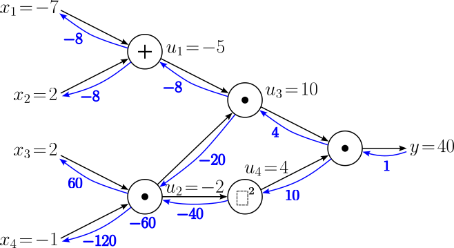
This leaves us with the final computational node to compute the last two gradients with respect to the last two remaining input variables $x_4$ and $x_5$. So one last time we apply the chain rule
$$ \begin{align} \large \frac{\partial y}{\partial x_3} &= \large \frac{\partial y}{\partial u_2}\cdot \frac{\partial u_2}{\partial x_3} \\[0.5em] \large \frac{\partial y}{\partial x_4} &= \large \frac{\partial y}{\partial u_2}\cdot \frac{\partial u_2}{\partial x_4} \\[0.5em] \end{align} $$Plugging in all the respective numbers gives us our final gradients.
$$ \begin{align} \large \frac{\partial y}{\partial x_3} &= \large -60\cdot x_4 = -60\cdot (-1) = 60 \\[0.5em] \large \frac{\partial y}{\partial x_4} &= \large -60\cdot x_3 = -60\cdot 2 = -120 \\[0.5em] \end{align} $$Now that we backpropagated through all nodes, we have completed the backward pass and have calculated all gradients. Let's have a look at the final computational graph.
Having gone through this more complex example in full detail, you might find it a bit tedious and boring since we have always performed the same basic steps for each operation (i.e., node in the computational graph). However, this is a good thing since this means that backpropagation is in its core quite simple and systematic, and therefore also rather straightforward to implement. Also appreciate that backpropagation does not only refer to the backward pass. While the backward pass requires some more careful consideration, the forward pass is crucial as it provides us with the intermediate results required to calculate the local gradients needed during the backward pass.
Summary
Backpropagation is a foundational algorithm in training artificial neural networks. It efficiently computes the gradients of a loss function with respect to the weights of the network, allowing the model to adjust its parameters to minimize prediction errors. At its core, backpropagation uses the chain rule of calculus to propagate errors backward through the network. The process begins with a forward pass, where inputs are passed through the network to generate predictions. A loss function then quantifies the difference between these predictions and the true labels. During the backward pass, gradients of the loss function are computed layer by layer, starting from the output layer and moving toward the input layer. These gradients indicate how each weight in the network should be adjusted to improve predictions.
The power of backpropagation lies in its ability to handle complex, multi-layer networks efficiently. Combined with optimization algorithms like stochastic gradient descent (SGD), it enables networks to learn from large datasets and improve iteratively. However, the algorithm requires careful initialization of weights and tuning of hyperparameters like the learning rate to avoid issues like vanishing or exploding gradients, which can impede training. Understanding backpropagation is essential for anyone working with deep learning models, as it provides insight into how networks learn and adapt. By grasping its mechanics, practitioners can better diagnose and troubleshoot training issues, optimize model performance, and innovate in neural network design.