Disclaimer: This Jupyter Notebook contains content generated with the assistance of AI. While every effort has been made to review and validate the outputs, users should independently verify critical information before relying on it. The SELENE notebook repository is constantly evolving. We recommend downloading or pulling the latest version of this notebook from Github.
Backpropagation (Generalization)
Backpropagation is a cornerstone algorithm in training neural networks, enabling them to learn from data by adjusting their parameters based on the gradient of a loss function. While the algorithm is often explained in the context of entire networks, it is fundamentally built upon the operation of individual computational nodes. Each node in a neural network performs a specific operation, such as addition, multiplication, or applying an activation function. By understanding how backpropagation works at the level of a single node, we can gain a deeper appreciation for how the algorithm scales to complex architectures.
At its core, backpropagation is a recursive application of the chain rule from calculus. For any given node in the computational graph, the algorithm calculates two key pieces of information: the forward pass output (the value computed by the node) and the backward pass gradient (how the loss changes with respect to the node's inputs). These gradients are propagated backward through the graph, allowing each node to contribute to the overall gradient computation. By isolating the mechanics of backpropagation at the level of a single node, we can generalize the process to any node type, whether it is performing a simple mathematical operation or a complex neural layer computation.
This tutorial will focus on generalizing backpropagation for a single computational node, breaking down its role in the larger graph. We will explore how to calculate local gradients, how to propagate those gradients to previous nodes, and how this process integrates into the broader framework of gradient descent. By the end, you will have a clear understanding of the principles that govern backpropagation and be able to apply this knowledge to various neural network configurations.
Preliminaries
Basic Notations
Throughout this notebook, we only consider a single computational node. However, this node can be part of an arbitrarily large computational graph. This node implements some function $f$ to calculate the output $u$ given some input $x$; more specifically:
y denotes the final output of a function or computational graph.
$x_1$, $x_2$, $x_3$,... denote input variable of a computational node; note that $x_i$ can be the input data or the output from some subsequent computational node; also, $x_i$ is not limited to be a scalar value but can also be a vector, matrix, or tensor.
$u$ denotes the results of a computational node implementing a function $f$.
Quick Recap: Chain Rule
The chain rule in calculus provides a way to compute the derivative of a composite function. Suppose $y$ depends on $u$, and $u$ in turn depends on $x$, i.e., $y=f(u)$ and $u=g(x)$. The chain rule states that the derivative of $y$ with respect to $x$ can be found by multiplying the derivative of $y$ with respect to $u$ by the derivative of $u$ with respect to $x$.
$$\large \frac{d y}{d x} = \frac{d y}{d u} \cdot \frac{d u}{d x} $$Here:
- $\large \frac{dy}{dx}$ is the rate of change of $y$ with respect to $x$,
- $\large \frac{dy}{du}$ is the rate of change of $y$ with respect to $u$,
- $\large \frac{du}{dx}$ is the rate of change of $u$ with respect to $x$.
Single Input & Single Output
The most basic case is a computation node that takes a single variable $x$ as input to calculate function $f$ to output its result $u$, and $u$ feeds only to a single other computational node. In the computational graph of a neural network, certain nodes typically have only a single input. These include:
Activation functions: Nodes that apply activation functions like ReLU, Sigmoid, Tanh, or others to the output of a linear transformation typically take a single input (e.g., the result of a weighted sum).
Unary element-wise operations: Such operations transform each element of a vector, matrix, or tensor individually, such as: exponential $exp(x)$, logarithm $\log{x}$, square root $x^2$, negation $-x$, etc.
Normalization layers: Normalization layers typically take a single input vector/matrix/tensor (though internally they may depend on additional learnable parameters or statistics).
Dropout layers: These layers apply stochastic dropout to individual inputs, acting as a filter with one input and one output.
Reshaping or resizing operations: Operations like reshaping or flattening tensors take a single input tensor and modify its shape.
Pooling layers: Pooling operations such as max pooling or average pooling typically take a single input vector/matrix/tensor.
In a computational graph, this node has a single incoming edge and a single outgoing edge.
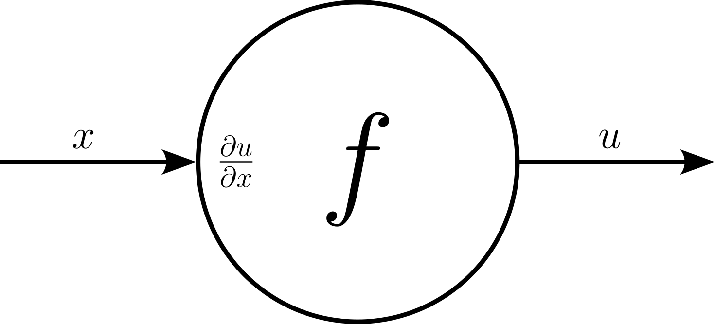
With only a single input, the computational node also has only a single local gradient $\large \frac{\partial u}{\partial x}$. For example let's assume that the node implements the simple function $u = f(x) = x^2$. This gives us a local gradient of ${\large \frac{\partial u}{\partial x}} = 2x$. During the forward pass, the node receives its input $x$ and can therefore calculate output $u$ as well as the local gradient. For example, assuming $x = 3$, we get $u = x^2 = 9$ and ${\large\frac{\partial u}{\partial x}} = 2x = 6$.
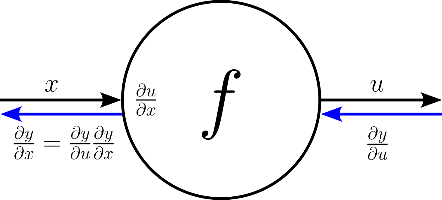
During the backward pass, the node will get the gradient $\large \frac{\partial y}{\partial u}$ that was backpropagated from the output to the node $f$. This gradient is commonly called the upstream gradient. Using the chain rule, we can node calculate $\large \frac{\partial y}{\partial x}$ as:
$$\large \large \frac{\partial y}{\partial x} = \frac{\partial y}{\partial u} \frac{\partial u}{\partial x} $$$\large \frac{\partial u}{\partial x}$ is commonly referred to as the downstream gradient. Visualized in our computational node:
To complete our example, if we assume a an upstream gradient ot ${\large \frac{\partial y}{\partial u}} = 0.5$, we can calculate the downstream gradient $\large \frac{\partial y}{\partial x}$ as:
$$\large \large \frac{\partial y}{\partial x} = \frac{\partial y}{\partial u} \frac{\partial u}{\partial x} = 0.5\cdot 6 = 3 $$Multiple Inputs & Single Output
Intuitively, computational nodes with two or more inputs are typically used for operations that combine multiple inputs or perform more complex computations. In a neural network, these commonly include:
Element-wise binary Operations: These operations combine vectors/matrices/tensors element-wise using common operations such as addition, subtraction, multiplication, division, maximum, minimum, etc.
Concatenation: Concatenation refers to combining multiple vectors/matrices/tensors along a specified dimension.
Vector/matrix/tensor multiplication: One of the most common operations in neural networks as they include the calculation of the weighted sums of inputs and learnable weights.
Gate Functions in RNNs: These functions combine the outputs from multiple inputs in Gated Recurrent Units (GRUs) or Long Short-Term Memory (LSTM) networks.
These are just some examples, as most operations in a neural network combine two or more outputs. Regarding the representation in a computation graph a operation that takes in multiple inputs is a node with multiple incoming edges.
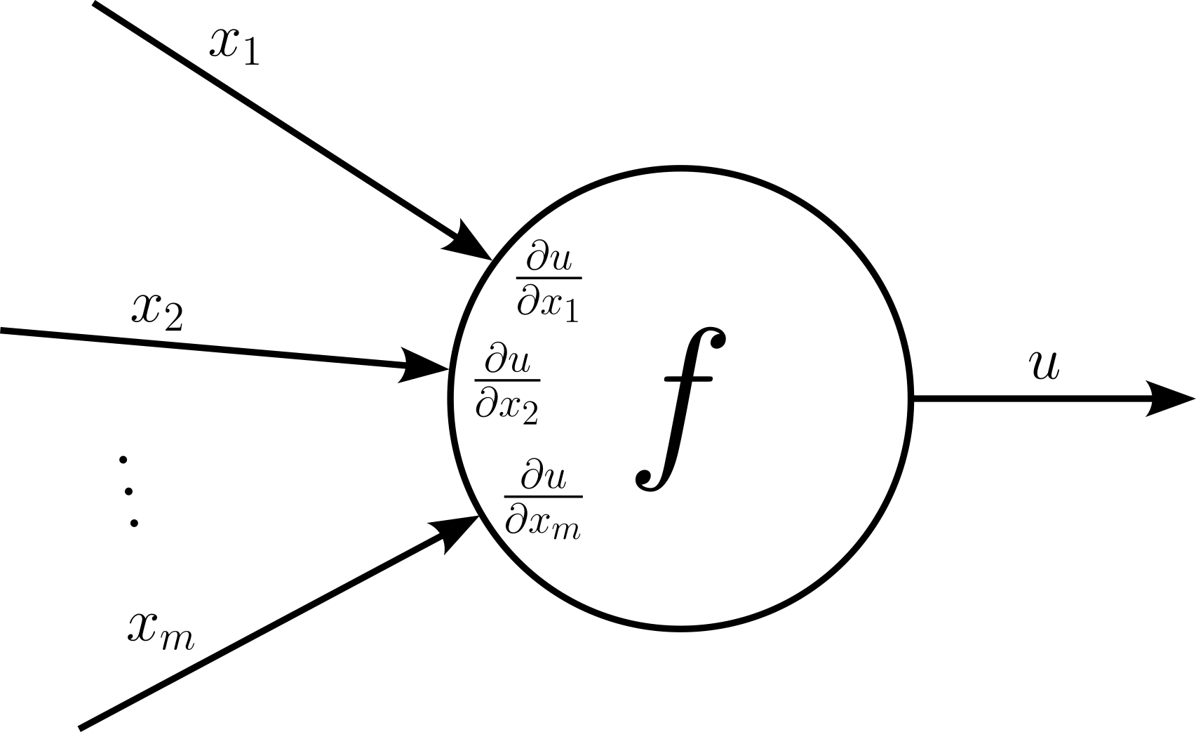
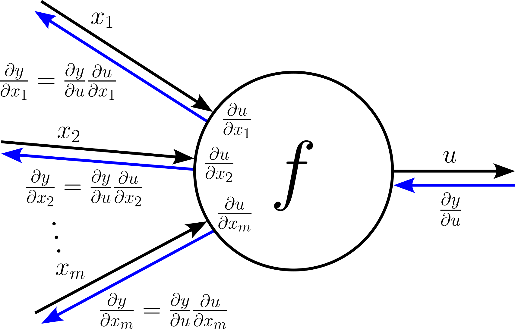
Each input $x_i$ maps to its own local gradient $\large \frac{\partial u}{\partial x_i}$. Otherwise, both the forward and the backward pass work exactly the same as for nodes with a single input. For one, this means that during the forward pass we can calculate the values for all local gradients $\large \frac{\partial u}{\partial x_i}$. During the backward pass, the node receives the upstream gradient $\large \frac{\partial y}{\partial y}$ which in turn allows to compute all downstream gradients $\large \frac{\partial x}{\partial x_i}$ as:
$$\large \large \frac{\partial y}{\partial x_i} = \frac{\partial y}{\partial u} \frac{\partial u}{\partial x_i} $$Again, let's visualize the backward flow of gradients through a node as part for a computational graph:
In short, the move from a single input to multiple inputs is very straightforward.
Multiple Inputs & Multiple Outputs
Apart from receiving multiple inputs, a node in a computational graph might return a result that is then used as input for more than one other node in the graph. Particularly in more advanced neural network architectures, this is a common occurrence; here are some popular examples:
Residual Connections: A residual connection is a key concept in neural network architectures, particularly introduced in Residual Networks (ResNets). They involve adding a "shortcut" or skip connection that bypasses one or more layers, allowing the input of a layer to be directly added to its output. This is mathematically expressed as $\mathbf{y}=F(\mathbf{x})+\mathbf{x}$, where $\mathbf{x}$ is the input to a layer, and $F(\mathbf{x}) is the transformation based on a subset of layers. In practice, residual connections are widely used in modern architectures like ResNet, Transformer models, and DenseNet variants, as they enable deeper networks to be trained effectively without performance degradation.
Inception Modules: Inception modules are a key building block in the Inception architecture (e.g., GoogleNet) designed to improve the efficiency and performance of convolutional neural networks (CNNs). The main idea of the Inception module is to capture features at multiple scales by applying different types of convolutional filters (e.g., $1\times 1$, $3\times 3$, $5\times 5$) and pooling operations in parallel on the same input. The outputs from these operations are then concatenated along the channel dimension to form a richer and more diverse feature representation. The Inception module allows the network to analyze spatial features at different scales simultaneously, improving its ability to detect patterns of varying sizes in the input data.
DenseNets: DenseNets (Dense Convolutional Networks) are a type of neural network architecture designed to improve feature propagation, encourage feature reuse, and reduce the number of parameters. DenseNets connect each layer to every other layer in a feed-forward fashion. Specifically, the output of each layer is concatenated with the outputs of all previous layers and used as input for subsequent layers. DenseNets are particularly useful for image classification and segmentation tasks, as they provide strong feature propagation and enable better gradient flow throughout the network.
Attention Mechanisms (Transformers): In Transformer architectures, outputs from a previous layer (e.g., the encoder output) are used in multiple heads of the multi-head attention mechanism. For example: the output of an encoder layer is split into queries (Q), keys (K), and values (V). These components are simultaneously used as input to multiple attention heads, where different projections are performed. Each head processes the input differently, but they all share the same source.
Multi-Task Learning: In multi-task learning, a shared backbone processes inputs, and the output of a shared layer serves as input to multiple task-specific layers. For example, a subnetwork of multiple convolutional layers may serve as the backbone to extract features from an image. The resulting feature map is then passed to (a) a classification head (e.g., for object recognition), (b) a bounding box regression head (e.g., for object detection), and (c) a segmentation head (e.g., for pixel-wise segmentation). Here, the shared backbone output is input to several task-specific layers.
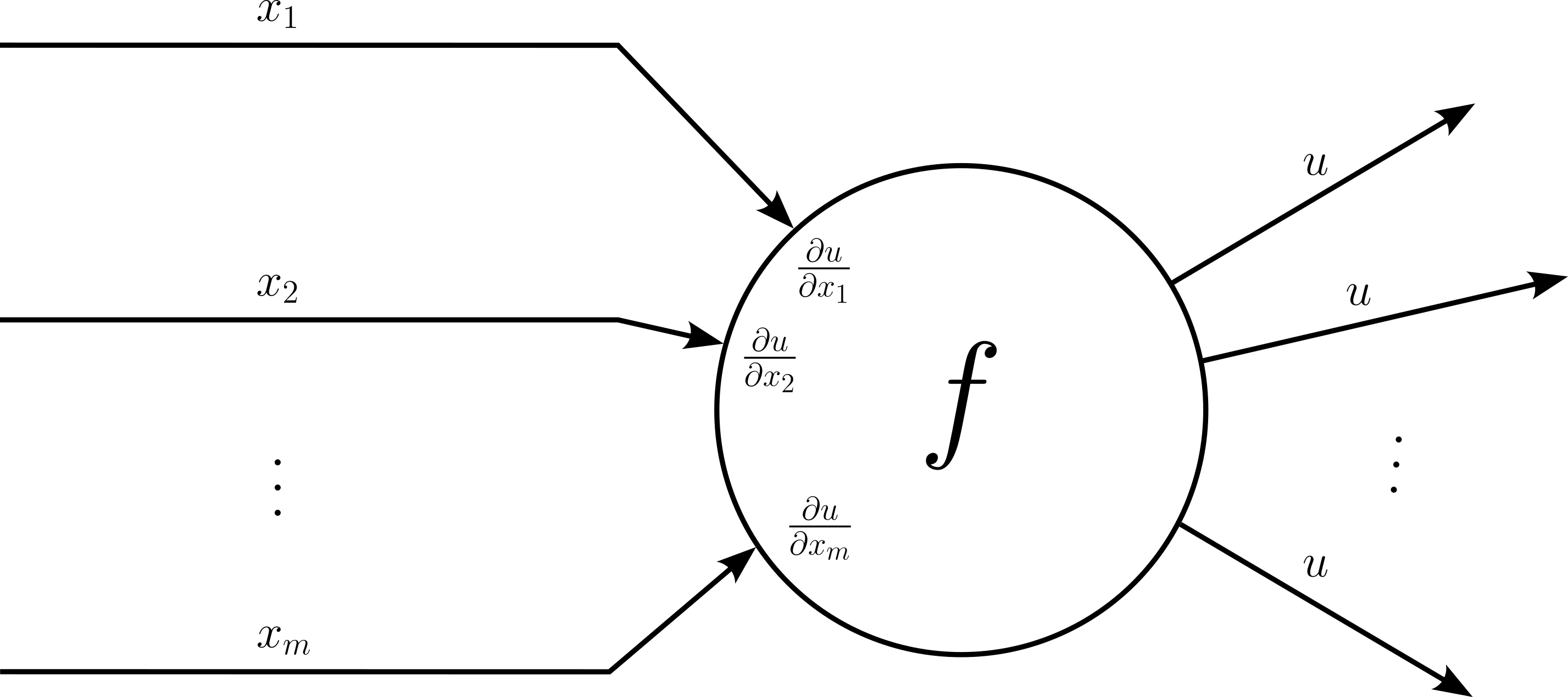
In terms of its representation in a computational graph, the re-use of a nodes' output is reflected by multiple outgoing edges, where each outgoing edge connects to a subsequent node. The example below shows a computational node receiving $n$ inputs and where its output $u$ feeds into $n$ other nodes in the computational graph.
Nodes with multiple outgoing edges — that is, nodes with an output that serves as input for multiple other nodes — adds an additional layer of complexity to the backpropagation process. Without such nodes, the computational graph is a tree with the final output as the root. In this case, there exists only a single path from the output to each input. Now, with nodes having multiple outgoing edges, there can be different paths from the output to an input. In this case, we need to apply the multivariable chain rule. Fortunately, this only means that we have to sum up all downstream gradients with respect to all upstream gradients.
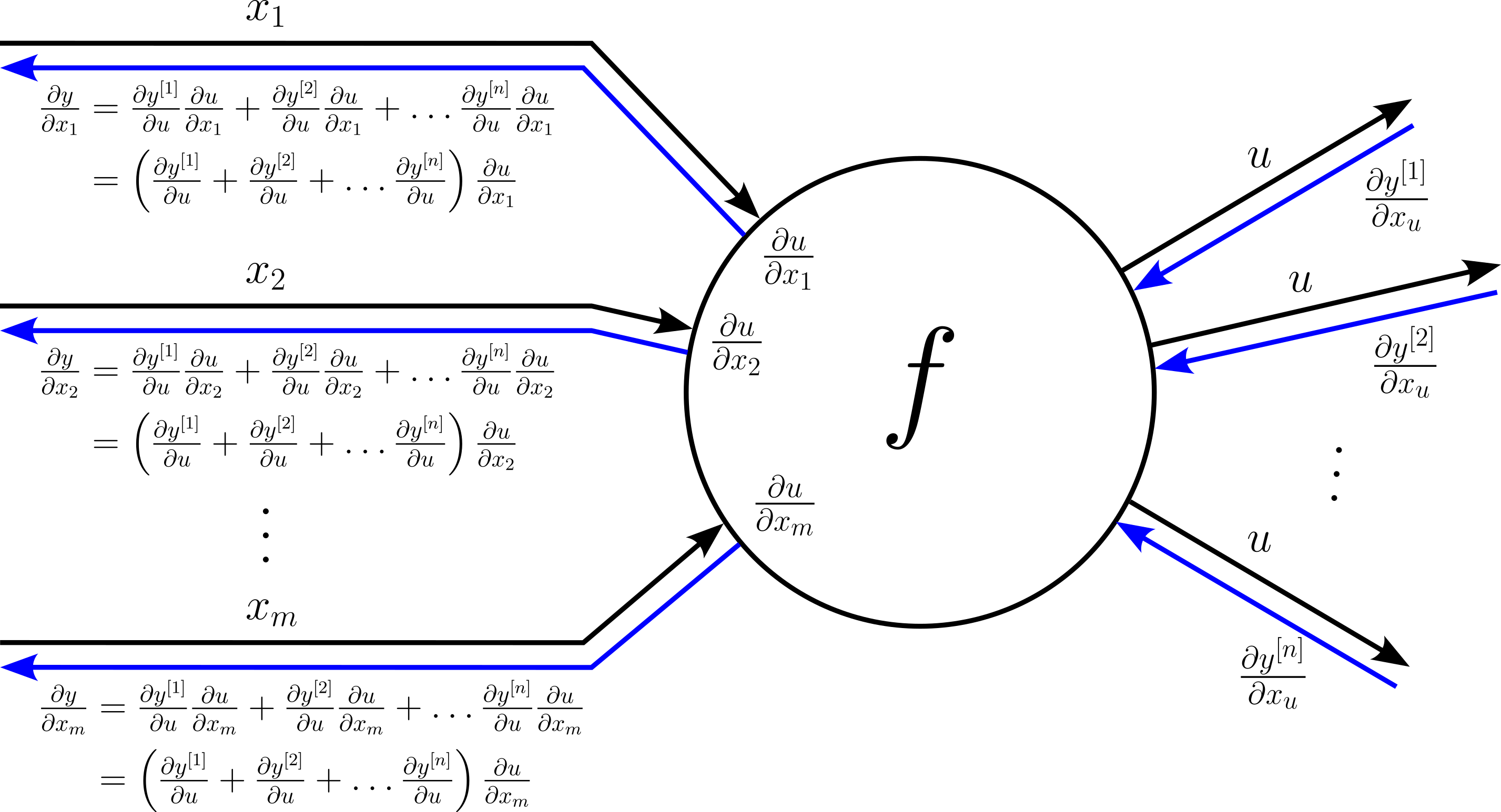
Let's assume our computational node feeds its output $u$ into $n$ other nodes. This mean, during the backward pass, the node will receive $n$ upstream gradients
$$ \large \frac{\partial y^{[1]}}{\partial u},\ \large \frac{\partial y^{[2]}}{\partial u},\ \dots,\ \large \frac{\partial y^{[n]}}{\partial u} $$When calculating the downstream gradient for each input $x_i$, we need to consider all upstream gradients by summing up all individual downstream gradients with respect to each upstream gradient; more specifically:
$$ \begin{align} \large \frac{\partial y}{\partial x_i} &= \large \frac{\partial y^{[1]}}{\partial u} \frac{\partial u}{\partial x_i} + \frac{\partial y^{[2]}}{\partial u} \frac{\partial u}{\partial x_i} + \dots \frac{\partial y^{[n]}}{\partial u} \frac{\partial u}{\partial x_i}\\[0.5em] &= \large \left( \frac{\partial y^{[1]}}{\partial u} + \frac{\partial y^{[2]}}{\partial u} + \dots \frac{\partial y^{[n]}}{\partial u} \right) \frac{\partial u}{\partial x_i} \end{align} $$Again, let's complete our picture of a computational node accordingly.
Summary
Backpropagation is a highly systematic process that leverages the chain rule from calculus to compute gradients efficiently in a computational graph. The ultimate goal is to determine how the loss function changes with respect to each parameter in the network. By decomposing this complex task into a series of smaller, more manageable steps, backpropagation systematically calculates gradients at every node in the graph. Each node’s gradient computation depends on two key components: the upstream gradients passed from subsequent nodes and the local gradients specific to that node’s operation.
The chain rule is the foundation of this process. For a function composed of multiple layers or operations, the derivative with respect to an input is the product of the derivatives of each intermediate operation. In backpropagation, this principle is applied recursively, starting from the loss function and moving backward through the network. At each node, the algorithm computes the local gradient, which quantifies the sensitivity of that node's output to its inputs. This local gradient is then multiplied by the upstream gradient—representing the influence of the subsequent nodes on the loss—yielding the downstream gradient. This multiplication ensures that every node contributes proportionally to the final gradient calculations.
What makes backpropagation particularly systematic is its modularity. Regardless of the operation performed by a node (e.g., addition, multiplication, or an activation function), the process of computing gradients remains consistent: calculate the local gradient, multiply by the upstream gradient, and propagate the result. This modularity allows backpropagation to adapt seamlessly to different node types and architectures, from simple feedforward networks to complex recurrent or convolutional models. Each node functions independently, relying only on its immediate neighbors in the graph, making the gradient computation both efficient and scalable.
Another key feature of backpropagation’s systematic nature is its ability to reuse intermediate results from the forward pass. During the forward pass, each node calculates and stores its output, which is then used in the backward pass to compute local gradients. This eliminates redundancy and ensures that gradients are computed efficiently without recalculating intermediate values. The combination of modular gradient computation and result reuse makes backpropagation a highly structured and computationally efficient algorithm.
Ultimately, the systematic approach of backpropagation ensures that the gradient for any parameter is calculated accurately and efficiently, even in large and complex networks. By propagating gradients backward using the chain rule, the algorithm maintains a clear flow of information from the loss function to each parameter, enabling effective learning through gradient descent. This consistency and scalability are what make backpropagation a cornerstone of modern deep learning.