Disclaimer: This Jupyter Notebook contains content generated with the assistance of AI. While every effort has been made to review and validate the outputs, users should independently verify critical information before relying on it. The SELENE notebook repository is constantly evolving. We recommend downloading or pulling the latest version of this notebook from Github.
Backpropagation Through Time (BPTT)
Backpropagation Through Time (BPTT) is the fundamental algorithm used to train Recurrent Neural Networks (RNNs) on sequential data. While many neural network architectures process inputs independently, RNNs are designed to handle sequences such as text, speech, or time series. In these settings, the output at each time step depends not only on the current input but also on the network’s internal state, which carries information from previous time steps. BPTT enables learning in this setting by extending the standard backpropagation algorithm so that gradients can be computed across multiple time steps of the sequence.
To understand BPTT, it is helpful to think of an RNN as being "unrolled" through time. Each time step corresponds to a copy of the same neural network, all sharing the same parameters. During training, the forward pass processes the sequence step by step, producing outputs and hidden states. BPTT then computes gradients by propagating the error backward through this chain of time steps. Because the same parameters are reused at every step, the gradients from all time steps are accumulated to update the shared weights. In this way, BPTT allows the model to learn how earlier inputs influence later predictions.
BPTT is considered a cornerstone for training RNNs because it enables the network to learn temporal dependencies, i.e, relationships between events that occur at different points in a sequence. For example, in language processing, the meaning of a word may depend on words that appeared many steps earlier. By propagating gradients through time, BPTT allows the model to adjust its parameters based on how earlier states contribute to later errors. Without BPTT, RNNs would not be able to effectively learn patterns that span multiple time steps.
What makes BPTT unique compared to training architectures such as feedforward neural networks, convolutional neural networks, or Transformers is the temporal dimension of gradient propagation. In feedforward models, gradients flow backward only through layers. In RNNs, gradients must flow both through layers and across time steps, often through long chains of repeated computations. This introduces additional challenges, such as vanishing or exploding gradients, which arise when gradients shrink or grow exponentially as they move through many time steps.
Understanding BPTT is important for anyone studying sequence modeling because it explains both the power and limitations of RNNs. Many important concepts (incl. truncated BPTT, gradient clipping, and the development of architectures like LSTMs and GRUs) are motivated by the challenges that arise when training with BPTT. Learning how BPTT works therefore provides deeper insight into how sequential neural networks learn from data and why certain architectural innovations were necessary to make sequence modeling practical.
Setting up the Notebook
This notebook does not contain any code, so there is no need to import any libraries.
Preliminaries
Before checking out this notebook, please consider the following:
The concept of fine-tuning is not limited to LLMs, and many of the covered techniques are model agnostic. However, fine-tuning became particularly important due to the popularity and extreme size of modern LLMs. Hence, most examples stem from the context of language modeling and related tasks.
This notebook is intended to serve as an introduction and overview to fine-tuning. While it covers the most common strategies for fine-tuning pretrained models, many more sophisticated and specialized strategies exist, but which would go beyond the scope of this notebook.
Quick Recap: Recurrent Neural Networks
Basic Architecture
Recurrent Neural Networks (RNNs) are are a class of neural network architectures specifically designed to handle sequential data, where the order of inputs matters. RNNs are therefore well suited for tasks involving sequences such as text, speech, and time series data. To capture the sequential nature of the data, we need to use a suitable representation to describe a data sample $\mathbf{x}$. The most common and straightforward way is describe a sample of sequential data as a list of the sequence elements:
where each element $\mathbf{x}_t$ is a feature vector — for example, the feature vector for time series data, word embedding vectors in case of text, image frames in case of video data, and so on. In this representation, $T$ marks the length of the sequence, and $\mathbf{x}_t$ marks the feature vector at time stamp $t$ — the notion of a time step is commonly used even for non-time series data such as words in a text or frame in a video.
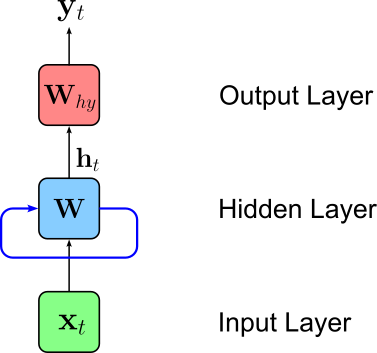
Each feature vector $\mathbf{x}_t$ is passed to the network one by one. However, we need some way for the network to "remember" some previous result from inputs $\mathbf{x}_1, \mathbf{x}_2, \dots, \mathbf{x}_{t-1}$ when processing $\mathbf{x}_t$. To accomplish this, RNNs introduce the concept of a hidden state. The hidden state is an additional vector incorporated into the network that commonly holds the output $\mathbf{h}$ of the hidden layer — although the hidden state can be arbitrarily further manipulated. As such, the size of the hidden state is typically simply the size of the hidden layer. With this hidden state the RNN retains information from previous time steps, allowing the model to capture dependencies in sequential data. Mathematically, the hidden state at time step $t$ can be expressed using the following recurrent formula:
In other words, the hidden state $\mathbf{h}_t$ at time step $t$ is some function of the hidden state $\mathbf{h}_{t-1}$ from previous timestamp $(t-1)$ and of the input feature vector $\mathbf{x}_t$ (e.g., a word embedding vector) at time step $t$. We can visualize this recurrent formula using our abstract representation of a neural network by adding adding a loop (blue edge) reflecting that the inputs of the hidden layers are now both the current input $\mathbf{x}_t$ and the previous output of the hidden layer retained by the hidden state.
To better visualize the sequential processing of the input and the evolution of the hidden state across all time steps, we can "unroll" our network architecture, to show the network at each time step and which inputs the hidden layer receives at each time step.
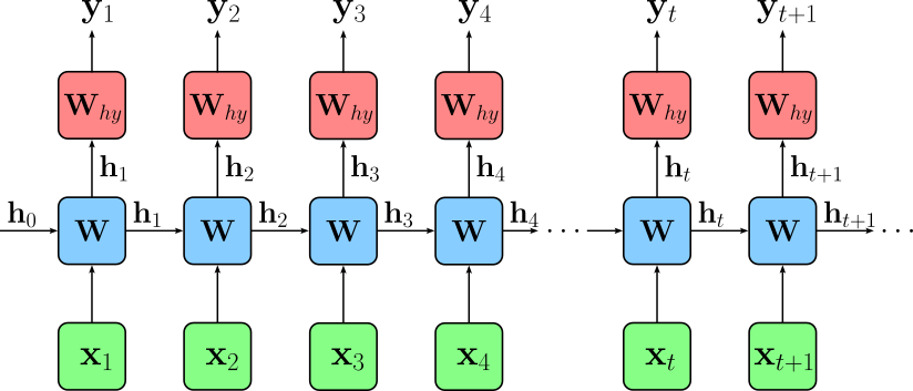
Note that we have to initialize the hidden state $\mathbf{h}_0$. A very basic approach is zero initialization where the initial hidden state is just a vector of zeros. While many other strategies exist, they are not relevant for our discussion here.
So far, we only considered the general form of the recurrent for $\mathbf{h}_t = f_{\mathbf{W}}(\mathbf{h}_{t-1}, \mathbf{x}_t)$. We still need to define how to implement the function $f_{\mathbf{W}}$. The simplest form of $f_{\mathbf{W}}$ that is commonly used in practice — therefore often also called Vanilla RNN — is implemented using the following function for $\mathbf{h}_t$ (function $f_y$ remains unchanged):
where $\mathbf{W}_{hh}$ and $\mathbf{W}_{xh}$ to are two weight matrices that transform the previous hidden state $\mathbf{h}_{t-1}$ and the current input vector $\mathbf{x}_t$, respectively. These weight matrices (and the bias vector $\mathbf{b}_h$) contain all trainable parameters of the hidden layer. Apart from increasing the capacity for the model to learn complex relationships, having both weight matrices also makes it easy to ensure that the results of $\mathbf{W}_{hh}\mathbf{h}_{t-1}$ and $\mathbf{W}_{xh}\mathbf{x}_{t}$ have the same size and can therefore be added.
Sequence Tasks & Losses
When training an RNN — like any other neural networks — we need to compute a loss by comparing the current predictions of our model with the ground truth given by our annotated dataset. In the case of an RNN, the predictions and therefore the loss we compute depends on the learning tasks. For example, when training a RNN for a sequence labeling task, the model produces an output at every time step of the input sequence, rather than a single prediction for the entire sequence. Each of these outputs corresponds to a label prediction for the respective time step (e.g., a tag for each word in a sentence). As a result, the training objective is defined over all time steps: a separate loss is computed by comparing each predicted output to its ground truth label; the figure below illustrates this setup.
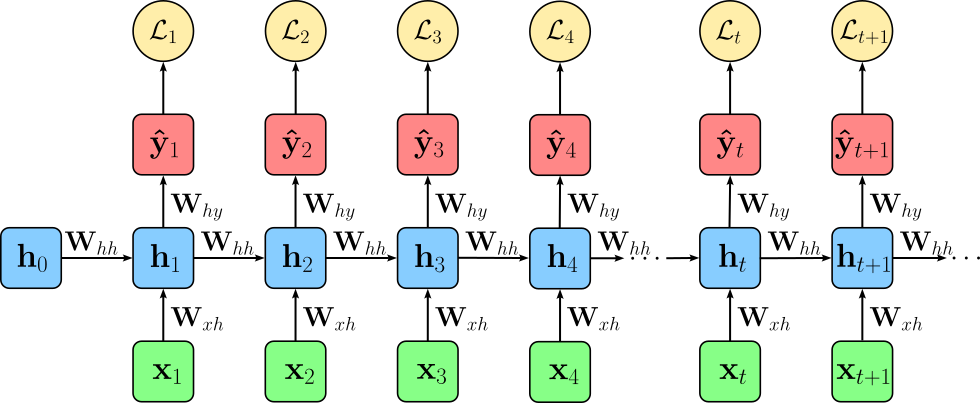
These individual losses are then aggregated, typically by summation or averaging, to form the total loss for the sequence. This setup ensures that the model learns to make accurate predictions at every position in the sequence, rather than focusing only on a final output. In short, we compute the total loss $\mathcal{L}$ for a training sample as:
In contrast, when training an RNN for a sequence-level classification task, the goal is to predict a single label for the entire sequence rather than labels for each time step. In this case, the RNN processes the sequence step by step, updating its hidden state, but only the output at the final time step is used for prediction. Consequently, the loss is computed solely with respect to this last output, comparing it to the ground truth label for the entire sequence. This approach allows the RNN to summarize the relevant information from the whole sequence into its final hidden state, which then drives the single classification decision. The figure below illustrates this setup; here, $T$ represents the lengths of the input sequence.
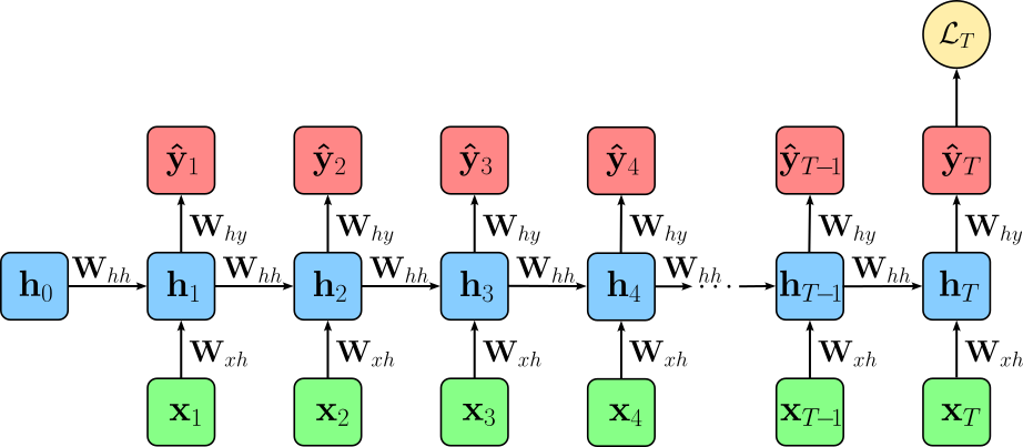
Thus, the total loss $\mathcal{L}$ for a training sample is simply the loss for the output of the last time step, i.e., $\mathcal{L} = \mathcal{L}_T$. In general, loss $\mathcal{L}$ may derive from other than all or only the last output of a sequence. However, the sequence labeling and the classification setup are by far the most common realizations.
Example Setup
The figure below shows the example setup we use through out this section to introcue the concept of BPTT. More specifically, we assume training an RNN for a classiciation tasks. As seen above, this means that we only compute the loss after processing the whole sequence for the last time step $T$. To make the example even more concrete, let $T=4$ (i.e., we have an input sequence of length $4$).
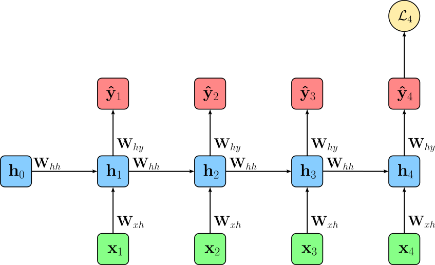
We choose this setup because it is simpler compared to training a sequence labeling task where we compute a loss $\mathcal{L}_t$ at each time step $t$. However, all the steps required to perform BPTT for a classification task can directly be extended to sequence labeling tasks, as we will show.
Training the RNN now means minimizing the loss, by performing backpropagation to compute the gradients with respect to all trainable parameters (i.e., mainly weights and biases) and updating these parameters. Recall that backpropagation computes the gradients of loss $\mathcal{L}$ with respect to its parameters in a systematic, step-by-step fashion. It works by applying the chain rule of calculus, which expresses the derivative of a composition of functions as a product of derivatives of the individual functions. In the context of a neural network, each layer can be viewed as a function that transforms its input into an output. Backpropagation starts at the output layer, computing the derivative of the loss with respect to the output, and then propagates these gradients backward through the network, layer by layer.
At each layer, the chain rule ensures that the gradient accounts for how changes in the layer's parameters affect not only its immediate output but also the subsequent layers all the way to the final loss. Specifically, it involves computing partial derivatives of the loss with respect to the layer's inputs, weights, and biases, multiplying them with the gradients received from the next layer. This accumulation of all partial derivatives guarantees that the final gradient for each parameter reflects its total influence on the loss, enabling accurate and efficient parameter updates during training. The figure below shows our example network with all partial derivatives between the layers (blue arrows).
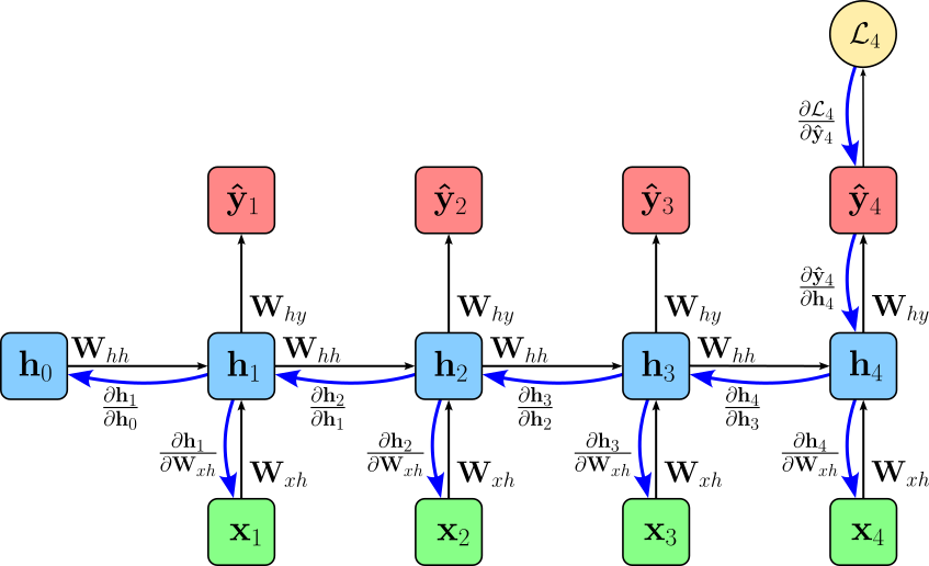
As we can see in this figure, backpropagation for RNNs is kind of unique because the hidden state at each time step depends not only on the current input but also on all previous hidden states. This temporal dependency means that when computing gradients during training, we cannot treat each time step independently like in a standard feedforward network. This is why we need to use Backpropagation Through Time (BPTT), which unrolls the RNN across all time steps and propagates the loss backward through the sequence. Each weight matrix is shared across time, so the gradients accumulate contributions from every time step where that weight was used. This is fundamentally different from feedforward networks, where each weight only affects one layer's output.
How BPTT Works
Let's dive into the inner workings of BPTT in a step-by-step manner. For this, we first need to look at the exact computations our example network is performing. Since we assume an input sequence of length $4$, we compute for hidden states $\mathbf{h}_{1}$, $\mathbf{h}_{2}$, $\mathbf{h}_{3}$, and $\mathbf{h}_{4}$. We then feed the last hidden state into a final output layer to map the hidden state to a vector $\mathbf{o}_{4}$ of size corresponding to the number classes in out classification task. Lastly, we apply the Softmax function to compute the output $\mathbf{\hat{y}}_{4}$ which converts vector $\mathbf{o}_{4}$ into a vector of output probabilities — for our example, we use that we use the Cross-Entropy Loss to compute loss $\mathcal{L}_{4}$. Using the implementation of the recurrent formula of a Vanilla RNN, all involved computations and parameters are:
To make our example more concrete, let's assume that we use this classification setup to training sentiment analysis model the predicts if an input text has "positive", "negative", or "neutral" sentiment. In this case, $\mathbf{x}_{i}\in \mathbb{R}^{e}$ are word embedding vectors of size $e$ (e.g., $e=300$, a common size of pretrained Word2Vec embeddings). The size of the hidden layer — and this each hidden state — is $h$ (e.g., $h=512$). Therefore, the recurrent formula contans the two weight matrices $\mathbf{W}_{xh}\in \mathbb{R}^{h\times e}$ and $\mathbf{W}_{hh}\in \mathbb{R}^{h\times h}$, as well as the bias vector $\mathbf{b}_{h}\in \mathbb{R}^{h}$. Assuming $c$ output classes (here: $c=3$) the output layer features the weight matrix $\mathbf{W}_{hy}\in \mathbb{R}^{c\times h}$ and the bias vector $\mathbf{b}_{y}\in \mathbb{R}^{c}$.
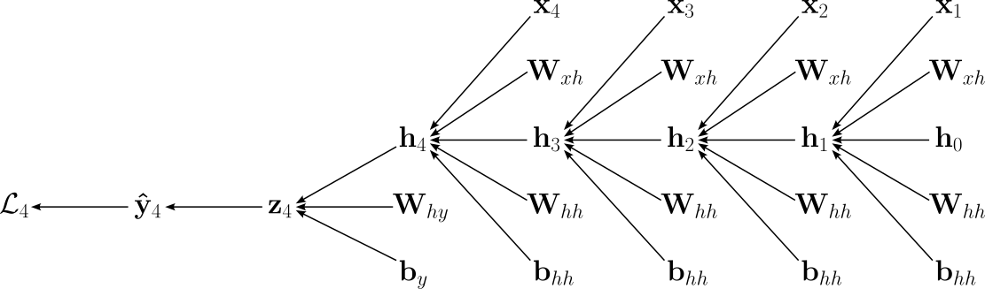
From this sequence of computations, we can see that the weight matrices $\mathbf{W}_{xh}$ and $\mathbf{W}_{hh}$ as well as the bias vector $\mathbf{b}_{h}$ influence the output $\mathbf{\hat{y}}_{4}$ and thus loss $\mathcal{L}_{4}$ multiple times. To make these dependencies even more explicit, the figure below shows the complete computational graph for computing $\mathcal{L}_{4}$. In this graph, an edge from a source to a target means that the source is an input for the function computing the target.
During training, the model now requires to compute all the gradients for the loss with respect to all trainable parameters. For our example network this includes:
- the gradients for the output layer: $\large \frac{\partial \mathcal{L}_{4} }{\partial \mathbf{W}_{hy}}$, $\large \frac{\partial \mathcal{L}_{4} }{\partial \mathbf{b}_{y}}$; and
- the gradients for the recurrent layer: $\large \frac{\partial \mathcal{L}_{4} }{\partial \mathbf{W}_{xh}}$, $\large \frac{\partial \mathcal{L}_{4} }{\partial \mathbf{W}_{hh}}$, $\large \frac{\partial \mathcal{L}_{4} }{\partial \mathbf{b}_{h}}$.
Let's see how we compute these gradients one by one using the computational graph shown above as a guide.
Gradients for Output Layer
Starting with the gradients of the output layer is reasonably straightforward since the two relevant parameters $\mathbf{W}_{hy}$ and $ \mathbf{b}_{y}$ appear only once in the computational graph. We can also see this when look only at computations for the last linear layer and the Softmax function:
Gradient with respect to Output Weights $\mathbf{W}_{hy}$
To compute $\large \frac{\partial \mathcal{L}_{4} }{\partial \mathbf{W}_{hy}}$, we apply the chain rule of calculus. The partial derivatives for the chain rule we get directly from the equations above or, even more easily from the computational graph. Thus, we have:
Note the partial derivatives of the Cross-Entropy Loss and the Softmax function are often combined because their composition leads to a remarkably simple and numerically stable gradient expression. When Softmax is used to convert logits into probabilities and Cross-Entropy is used as the loss, applying the chain rule causes many terms in the Jacobian of Softmax to cancel with terms from the loss derivative. Combine both partial derivatives gives us:
By combining both partial derivatives, the gradient $\large \frac{\partial \mathcal{L}_4}{\partial \mathbf{z}_4}$ simplifies to $\left(\mathbf{\hat{y}}_4 - \mathbf{y}_{4} \right)$, avoiding the need to explicitly compute the full Jacobian matrix of Softmax, which would be computationally expensive. This simplification not only makes backpropagation more efficient but also improves numerical stability, since working directly with logits and this compact gradient reduces issues like overflow or underflow that can arise when handling exponentials separately. We discuss this behavior of the Softmax function together with the Cross-Entropy loss in full detail in a separate notebook. After inserting the the gradient, we get:
Computing $\large \frac{\partial \mathbf{z}_4}{\partial \mathbf{W}_{hy}}$ is equally straightforward since we have a simple linear layer $\mathbf{W}_{hy}\mathbf{h}_4 + \mathbf{b}_y$ which gives us $\large \frac{\partial \mathbf{z}_4}{\partial \mathbf{W}_{hy}} = \mathbf{h}_{t}$ — again, we formally derive all partial derivatives involved in a linear layer in a separate notebook. This means we can now compute the partial derivative $\large \frac{\partial \mathcal{L}_{4} }{\partial \mathbf{W}_{hy}}$ as:
So far, we explicitly consider the loss $\mathcal{L}_4$ as the loss for the last time step for an input sequence of length $4$. Of course, we can generalize this to the loss with respect to any time step $t$, with $1\leq t \leq T$:
Furthermore, we can also extend to computation also to a sequence labeling task where we need to sum up the gradients with respect to all losses:
Gradient with respect to Output Bias $\mathbf{b}_{y}$
Computing $\large \frac{\partial \mathcal{L}_{4} }{\partial \mathbf{b}_{y}}$ is equally straightforward since we are basically performing the exact same steps. Firstly, we apply the chain rule the get the product of partial derivatives of the individual functions we have in the computational graph:
Again, by combining the partial derivatives for the Cross-Entropy Loss and the Softmax function to $\large \frac{\partial \mathcal{L}_4}{\partial \mathbf{z}_4}$, we get the same simple and numerically stable gradient expression:
Given the linear layer $\mathbf{W}_{hy}\mathbf{h}_4 + \mathbf{b}_y$, the gradient $\large \frac{\partial \mathbf{z}_4}{\partial \mathbf{b}_{y}}$ simply becomes $1$, giving us:
Generalizing to any time step $t$, we get:
And lastly, we can again extend this computation to sequence labeling task where we need to sum up the gradients with respect to all time steps:
Gradient with respect to Last Hidden State $\mathbf{h}_{4}$
Apart from the weight matrix $\mathbf{W}_{hy}$ and the bias vector $ \mathbf{b}_{y}$, we also have to the last hidden state $\mathbf{h}_{4}$ that affects the computation of the loss as the input of the linear output layer. As such, we once more apply the chain rule of calculus to express the gradients as the product of the respective partial derivatives:
We already saw how we can combine the Cross-Entropy Loss and Softmax function to get a simple expression for their combined gradient:
Using the "rules" for computing the partial derivatives for a linear layer — you can check out the dedicated notebook for full details, we get the following final expression to compute $\large \frac{\partial \mathcal{L}_{4} }{\partial \mathbf{h}_{4}}$:
We could generalize this expression to $\large \frac{\partial \mathcal{L}_{t} }{\partial \mathbf{h}_{t}}$, but we address this when we cover the recurrent layer as whole in the next section.
Note that all previous expressions for the gradients for the output layer look very simple since we only assume a single linear layer as the output layer. Of course, the hidden state $\mathbf{h}_t$ may be fed into more than one linear output layer. However, despite this added complexity, the gradient computation remains conceptually straightforward because these output layers form a standard feed-forward subnetwork without any temporal dependencies. This means we can compute their gradients using the familiar layer-by-layer backpropagation rules from feed-forward networks, and simply aggregate their contributions before passing gradients back into the recurrent hidden state.
Gradients for Recurrent Layer
Computing the gradients $\large \frac{\partial \mathcal{L}_{4} }{\partial \mathbf{W}_{xh}}$, $\large \frac{\partial \mathcal{L}_{4} }{\partial \mathbf{W}_{hh}}$, and $\large \frac{\partial \mathcal{L}_{4} }{\partial \mathbf{b}_{h}}$ are now more interesting since the weight matrices $\mathbf{W}_{xh}$ and $\mathbf{W}_{hh}$ as well as the bias vector $\mathbf{b}_{h}$ in the recurrent layer are used multiple times to compute the loss. In the following, we focus on computing $\large \frac{\partial \mathcal{L}_{4} }{\partial \mathbf{W}_{xh}}$; the solutions for $\large \frac{\partial \mathcal{L}_{4} }{\partial \mathbf{W}_{hh}}$, and $\large \frac{\partial \mathcal{L}_{4} }{\partial \mathbf{b}_{h}}$ are then straightforward.
Gradient with respect to Input-to-Hidden Weights $\mathbf{W}_{xh}$
To compute the gradient of the loss with respect to the input-to-hidden weight matrix $\mathbf{W}_{xh}$, let's look again at the computation graph, but now specifically consider the multiple different backward passes from loss $\mathcal{L}_{4}$ to the $4$ usages of $\mathbf{W}_{xh}$; see the figure below, where the $4$ different paths reflecting the $4$ time steps are color-coded.
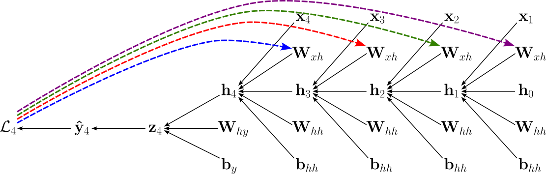
In calculus, when a variable influences an output through multiple computational paths, all of these paths must be taken into account when computing derivatives. This follows directly from the multivariable chain rule: each path contributes a partial derivative, and the total effect is obtained by summing these contributions. Intuitively, if a change in an input can propagate through different routes in a computation graph, each route carries part of the influence, and ignoring any of them would underestimate the true sensitivity of the output with respect to that input.
This principle applies here, where branching structures are a result from the recurrent connections. Whenever a signal splits and later recombines, the gradient flowing backward must also split and then be summed at the merging point. As a result, the total gradient with respect to a variable is the sum of gradients from all downstream paths, ensuring that every way in which the variable affects the output is properly accounted for. Thus, $\large \frac{\partial \mathcal{L}_4 }{\partial \mathbf{W}_{xh}}$ is therefore computed as the sum of $4$ expression using the chain rule, with each expression representing on of the paths. The partial derivatives of the multiple chain rule expressions can be directly inferred from the computational graph. In the formula below, we color each of the $4$ expressions to match the color-coded paths in the figure above.
Just from this formula for an input sequence of length $4$, we can see how it would extend for longer sequences by adding more partial derivatives of the form $\large \frac{\partial{\mathbf{h}_{j}}}{\partial\mathbf{h}_{j-1}}$. Let's combine these partial derivatives into their own product, first using our concrete example of a sequence with length $4$. We can therefore rewrite the previous formula as:
This now allows us to generalize this formula for losses at any time step $t$:
When looking at this formula, we already know how to compute $\large \frac{\partial \mathcal{L}_{t} }{\partial \mathbf{h}_{t}}$, but we still need to figure out how to compute $\large \frac{\partial{\mathbf{h}_{j}}}{\partial\mathbf{h}_{j-1}}$ and $\large \frac{\partial \mathbf{h}_k}{\partial \mathbf{W}_{xh}}$ To compute the the derivative $\large \frac{\partial{\mathbf{h}_{j}}}{\partial\mathbf{h}_{j-1}}$, let's break it down into two parts:
How the activation changes with respect to the pre-activation: $\large \frac{\partial{\mathbf{h}_{j}}}{\partial\mathbf{o}_{j}}$, where $\mathbf{o}_{t} = \mathbf{W}_{hh}\mathbf{h}_{j-1} + \mathbf{W}_{xh}\mathbf{x}_{j} + \mathbf{b}_h$
How the pre-activation changes with respect to the previous hidden state: $\large \frac{\partial\mathbf{o}_{j}}{\partial\mathbf{h}_{j-1}}$
In other words, we can write:
For the pre-activation, since $\mathbf{o}_{j} = \mathbf{W}_{xh}\mathbf{h}_{t-1} + (\text{terms independent of }\mathbf{h}_{j-1})$, the derivative with respect to $\mathbf{h}_{t−1}$ is simply the weight matrix — again, this directly derives from the derivatives of a linear layer detailed in a separate notebook — giving us:
Regarding the activation, $\large \frac{\partial{\mathbf{h}_{j}}}{\partial\mathbf{o}_{j}}$ is the derivative of the element-wise activation function $\phi$. Since $\phi$ is applied to each element of the vector $\mathbf{o}_{j}$ independently — the $k$-th output of the activation function only depends on the $k$-th input — its derivative (i.e., the Jacobian) is a diagonal matrix:
where $\phi^\prime$ is the derivative of activation $\phi$. In case of a Vanilla RNN, the activation function is the $\tanh$ function where:
The derivative of the $\tanh$ function is:
Since in our case $x$ is the pre-activation signal $\mathbf{o}_j$ and $\mathbf{h} = \tanh(\mathbf{o}_j)$, we get the simple expression:
Thus, putting everything together, we can compute $\large \frac{\partial{\mathbf{h}_{j}}}{\partial\mathbf{h}_{j-1}}$ as follows:
The last remaining gradient to compute is $\large \frac{\partial \mathbf{h}_k}{\partial \mathbf{W}_{xh}}$. Again, if we split the computation into the partial derivative $\large \frac{\partial{\mathbf{h}_{j}}}{\partial\mathbf{o}_{j}}$ with respect to the pre-activation and the partial derivative $\large \frac{\partial\mathbf{o}_{j}}{\partial\mathbf{h}_{j-1}}$, we get:
We already know the expression for $\large \frac{\partial{\mathbf{h}_{k}}}{\partial\mathbf{o}_{k}}$ which here is $\text{diag}\left(1 - \mathbf{h}_k^2 \right)$. To compute $\large \frac{\partial\mathbf{o}_{k}}{\partial\mathbf{W}_{xh}}$, we again can use the fact that the recurrent function is basically a linear layer — even though we have two weight matrices here — to get:
This now gives us the complete expression to compute $\large \frac{\partial \mathbf{h}_k}{\partial \mathbf{W}_{xh}}$:
Finally, after so many tedious steps, we have all the parts to compute the gradient for the loss with respect to the input-to-hidden weight matrix $\mathbf{W}_{xh}$:
Like before, we can also extend this formula to sum up the gradients of all $T$ losses with respect to $\mathbf{W}_{xh}$ in the case of sequence labeling tasks.
This complete formula looks arguably quite scary. However, as we will later discuss in more detail, do not directly implement this formula as it is computationally prohibitive and numerically unstable. For example, explicitly calculating the nested product of Jacobians $(\prod \text{diag}(1 - h_i^2) W_{xh}^T)$ for every time step would require $O(T^2)$ operations, making training crawl as sequence lengths increase. Furthermore, the repeated multiplication of the weight matrix and the $\tanh$ derivative leads to the infamous vanishing and exploding gradient problems, where the error signal either dissipates into insignificance or grows to infinity before it can reach the early parts of the sequence.
Gradient with respect to Hidden-to-Hidden Weights $\mathbf{W}_{hh}$
Computing the gradient with respect to $\mathbf{W}_{hh}$ involves essentially the exact same step we have just seen since the backward passes are almost identical, given the simple recurrent formula of the Vanilla RNN implementation. More specifically, the gradient of loss $\mathcal{L}$ with respect to $\mathbf{W}_{hh}$ is:
The only component that is different is that we now need to compute $\large \frac{\partial \mathbf{h}_k}{\partial \mathbf{W}_{hh}}$ here. But still, this computation is also analogous to computing $\large \frac{\partial \mathbf{h}_k}{\partial \mathbf{W}_{xh}}$ as seen before and giving us:
Plugging this gradient and the ones we already know gives us again all expressions to compute $\large \frac{\partial \mathcal{L}_{t} }{\partial \mathbf{W}_{hh}}$ and $\large \frac{\partial \mathcal{L} }{\partial \mathbf{W}_{xh}}$ like before; we therefore omit them here.
Gradient with respect to Hidden Bias $\mathbf{b}_{h}$
The last gradient we need to compute is with respect to the bias vector $\mathbf{b}_{h}$. However, once again, given the simple implementation of the Vanilla RNN, we almost get the same expression for $\large \frac{\partial \mathcal{L}_{t} }{\partial \mathbf{b}_{h}}$ as for the the two weight matrices $\mathbf{W}_{xh}$ and $\mathbf{W}_{hh}$:
Here, the new component is not the partial derivative $\large \frac{\partial \mathbf{h}_k}{\partial \mathbf{b}_{h}}$. When following the same steps as done previously, we need to compute $\large \frac{\partial \mathbf{o}_{k}}{\partial \mathbf{b}_{h}}$, which is simple the identity matrix $\mathbf{I}$. Thus, we can compute $\large \frac{\partial \mathcal{L}_{t} }{\partial \mathbf{b}_{h}}$ simply as:
With this, we now have all the formulas to compute the gradient of the loss function with respect to all the trainable parameters in the network. It is rather clear for the various expressions that BPTT adds a significant complexity to the idea of backpropagation as seen in simple feed-forward neural networks — although all underlying concepts remain exactly the same. This added complexity also poses additional challenges when it actually comes to implementing BPTT as well as addressing potentially "problematic" behavior of the gradients. We outline these challenges in the next section.
Discussion — Challenges & Extensions
The purpose of this notebook is to introduce BPTT and how the recurrent nature of RNNs influences the computation of all gradients required when training an RNN-based model. As a result, we now also have all the formulas to compute the gradients for a Vanilla RNN. While this lays the most important foundation, actually implementing and using BPTT for training raises additional issues. In the following, we briefly motivate and outline these issues on a fairly high level, but keep in mind that more detailed discussion would go way beyond the scope of this notebook.
Practical Implementation
All the unrolled formulas derived from the unrolled computational graph we have seen to compute all required gradients for BPTT are expressed as a sum over all time steps with long chains of Jacobian products. While this representation is mathematically explicit and useful for understanding how information flows backward through time, it quickly becomes impractical for implementation. The number of terms grows linearly with the sequence length, and each term itself contains products of multiple matrices, making the expressions both computationally expensive and difficult to manage in code; more specifically, there are two main considerations:
Redundancy. In the unrolled formulas, many intermediate quantities (e.g, the partial derivatives $\large \frac{\partial{\mathbf{h}_{j}}}{\partial\mathbf{h}_{j-1}}$ of hidden states with respect to earlier states—are recomputed multiple times. This leads to significant inefficiency, especially for long sequences. In practice, we instead exploit the recursive structure of recurrent neural networks by reusing previously computed gradients. Dynamic programming allows us to cache intermediate results (e.g., the gradient with respect to the hidden state at time step $t$) and reuse them when computing gradients for earlier time steps, reducing both computation and memory overhead.
Numeric Stability. The unrolled expressions involve long products of Jacobians, which can easily lead to vanishing or exploding gradients; see below. While this issue is inherent to RNNs themselves, explicitly computing long chains of matrix products as suggested by the unrolled formulas can exacerbate numerical instability. Recursive implementations help mitigate this by organizing computations step by step, often combined with practical techniques like gradient clipping or truncated BPTT to further stabilize training.
Modern machine learning frameworks such as PyTorch or Tensorflow are built around automatic differentiation, which naturally implements backpropagation in a recursive, graph-based manner rather than through explicit unrolled formulas. These systems construct a computational graph during the forward pass and then traverse it backward efficiently, applying the chain rule locally at each operation. This approach avoids the need to manually encode the full unrolled expressions while still computing exactly the same gradients, making it both more efficient and less error-prone in practice.
Vanishing & Exploding Gradients
To better understand the problem, let's have another look at are unrolled formula for computing the gradients using the weight-to-hidden matrix as an example:
The part that poses the most challenges is the product which depends on the length of the input sequence. Each term in this product, $\large \frac{\partial{\mathbf{h}_{j}}}{\partial\mathbf{h}_{j-1}}$, is a Jacobian matrix containing the partial derivatives of the current hidden state $\mathbf{h}_{j}$ with respect to the previous one $\mathbf{h}_{j-1}$. In a standard RNN, this transition usually involves a weight matrix $\mathbf{W}_{hh}$ and an activation function $\phi$ (e.g., $\tanh$ in the case of a Vanilla RNN). We already know that we can compute this Jacobian as $\text{diag}\left(\phi^\prime(\mathbf{o}_{j}) \right)\mathbf{W}_{hh}^{\top}$ which gets repeatedly multiplicated as when computing the product term. This can lead two fundamental problems:
Vanishing Gradients. If the weights in $\mathbf{W}_{hh}$ are small and/or the activation function's derivative is small (as is common with $\tanh$ where the derivative is $\leq 1$), the product shrinks exponentially toward zero. By the time the gradient "reaches" the earliest time steps, it is so tiny that the weights for those steps are never effectively updated, meaning the model cannot learn long-term dependencies.
Exploding Gradients. In contrast, if the weights in $\mathbf{W}_{hh}$ are large the product of these Jacobians grows exponentially as the number of time steps increases. This causes the gradient values to "explode", making the weight updates so large that the model fails to converge.
To minimize the risk of vanishing and exploding gradients, the general goals is to maintain the weight matrix $\mathbf{W}_{hh}$ in a "healthy" range, primarily using sophisticated initialization schemes and regularization techniques. Beyond direct weight manipulation, other structural and algorithmic countermeasures are essential for stabilizing RNNs. Gradient Clipping is a widely used "safety net" that rescales gradients if their norm exceeds a predefined threshold, preventing the optimization from jumping into unstable regions of the loss surface. However, more fundamentally, the transition from Vanilla RNNs to gated architectures like LSTMs and GRUs is the most effective countermeasure; these units use an internal "cell state" with additive update rules that allow gradients to flow through time without being repeatedly multiplied by the same weight matrix. So let's look at these RNN variants a bit more closely
Beyond Vanilla RNN: LSTM & GRU
In this notebook we considered what we called a Vanilla RNN based on its simple realization of the recurrent formula, where we compute the hidden state $\mathbf{h}_{t}$ at time step $t$ as $\mathbf{h}_t = \tanh{\left( \mathbf{W}_{hh}\mathbf{h}_{t-1} + \mathbf{W}_{xh}\mathbf{x}_{t} + \mathbf{b}_h \right)}$. The figure below shows a common visual representation of this implementation side by side with the formula. Note that this representation shows how different inputs are combined and which operations (incl. activation functions) are applied; however, the representation omits any weight matrices and bias vectors to keep it simple.
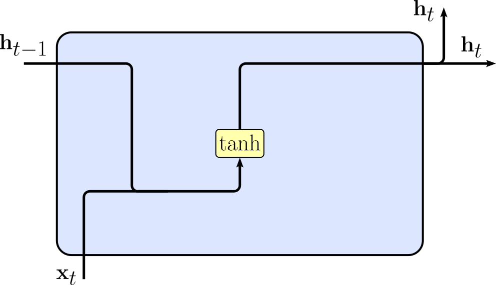 |
$$\large \mathbf{h}_{t} = \tanh{\left( \mathbf{W}_{hh}\mathbf{h}_{t-1} + \mathbf{W}_{xh}\mathbf{x}_{t} + \mathbf{b}_h \right)}$$ |
We also just saw how this basic implementation may suffer from vanishing and exploding gradients because of this purely multiplicative structure if the weight matrix $\mathbf{W}_{hh}$ is not maintained in a healthy range. More sophisticated RNN variants improve on this by adding additive update paths. In simple terms, the fundamental benefit of these additive update paths is that they create a "linear highway" for gradients to flow across time or layers without being exponentially transformed. In a multiplicative system, the gradient of the current state with respect to a much earlier state is a product of many Jacobian matrices. In an additive system, the gradient is a sum of terms, which is much more numerically stable. Let's briefly look at the two most popular RNN variants.
Firstly, a Long Short-Term Memory (LSTM) is a special type of recurrent neural network designed to remember information over long sequences. Beyond just the hidden state $\mathbf{h}_{t}$, an LSTM has a memory cell state $\mathbf{c}_{t}$ and gating mechanisms that control how information is stored, updated, or forgotten. The gates — called the input gate, forget gate, and output gate* — allow the network to decide what to keep from the past, what new information to add, and what to use as output. The figure below visualizes how an LSTM implements the recurrent formula, which is not much more complex compared to an RNN; note that a deeper understanding of all expressions is beyond our scope here and not required for our discussion.
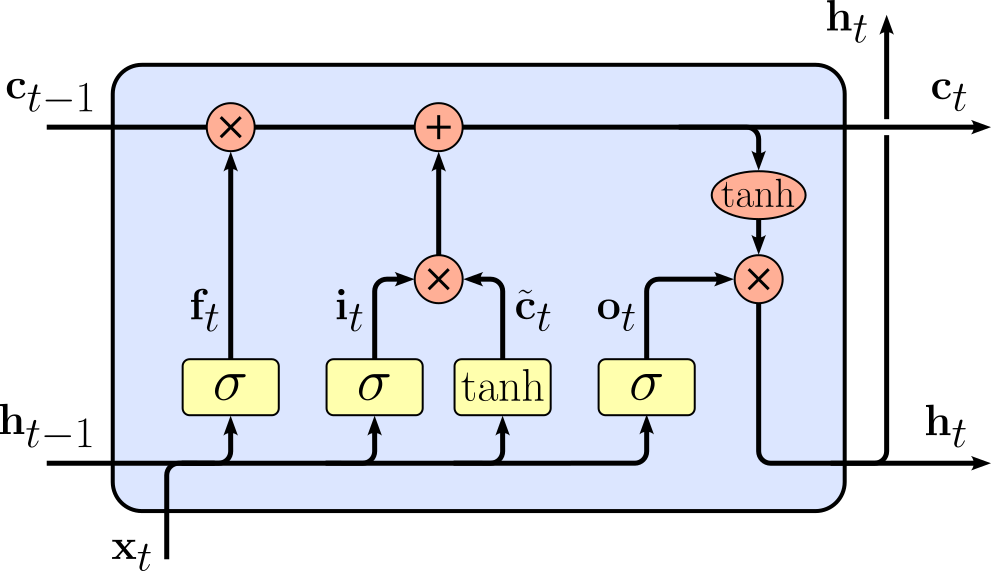 |
$$\begin{align} \large \mathbf{f}_t\ &\large = \sigma(\mathbf{W}_f x_t + \mathbf{U}_f \mathbf{h}_{t-1} + \mathbf{b}_f)\\[1em] \large \mathbf{i}_t\ &\large = \sigma(\mathbf{W}_i \mathbf{x}_t + \mathbf{U}_i \mathbf{h}_{t-1} + \mathbf{b}_i)\\[1em] \large \mathbf{\tilde{c}}_t\ &\large = \tanh(\mathbf{W}_c \mathbf{x}_t + \mathbf{U}_c \mathbf{h}_{t-1} + \mathbf{b}_c)\\[1em] \large \mathbf{c}_t\ &\large = \mathbf{f}_t \odot \mathbf{c}_{t-1} + \mathbf{i}_t \odot \tilde{c}_{t}\\[1em] \large \mathbf{o}_t\ &\large = \sigma(\mathbf{W}_o \mathbf{x}_t + \mathbf{U}_o \mathbf{h}_{t-1} + \mathbf{b}_o)\\[1em] \large \mathbf{h}_t\ &\large = \mathbf{o}_t \odot \tanh(\mathbf{c}_t) \end{align} $$ |
The important observation here is the inclusion of additive update paths which lets LSTMs carry important information across many time steps without it vanishing or exploding.
Secondly, like an LSTM, a Gated Recurrent Unit (GRU) is designed to (better) handle long-term dependencies in sequences compared to Vanilla RNNs. Like LSTMs, GRUs use gates to control the flow of information, but they are simpler in structure. A GRU combines the functions of the LSTM's input and forget gates into a single update gate and uses a reset gate to decide how much past information to forget when computing the new candidate state. Because of this, GRUs have fewer parameters than LSTMs, which can make them faster to train while still being effective at capturing dependencies across time steps. Again, we visualize the implementation of a GRU and show the involved computations below.
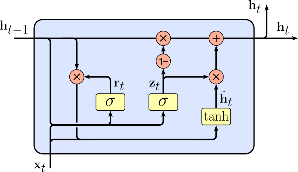 |
$$\begin{align} \large \mathbf{z}_t\ &\large = \sigma(\mathbf{W}_z \mathbf{x}_t + \mathbf{U}_z \mathbf{h}_{t-1} + \mathbf{b}_z)\\[1em] \large \mathbf{r}_t\ &\large = \sigma(\mathbf{W}_r \mathbf{x}_t + \mathbf{U}_r \mathbf{h}_{t-1} + \mathbf{b}_r)\\[1em] \large \mathbf{\tilde{h}}_t\ &\large = \tanh(\mathbf{W}_h \mathbf{x}_t + \mathbf{U}_h (\mathbf{r}_t \odot \mathbf{h}_{t-1}) + \mathbf{b}_h)\\[1em] \large \mathbf{h}_t\ &\large = (1 - \mathbf{z}_t) \odot \mathbf{h}_{t-1} + \mathbf{z}_t \odot \mathbf{\tilde{h}}_t \end{align} $$ |
Compared to LSTMs, GRUs are generally lighter and simpler, but they still benefit from the same fundamental idea: additive update paths that allow gradients to flow more easily, avoiding vanishing or exploding gradients. While LSTMs may perform slightly better on very long sequences due to their separate memory cell and output gate, GRUs often achieve similar performance on many tasks with less computational cost. Essentially, GRUs strike a balance between model complexity and sequence learning capability, making them a popular alternative to LSTMs.
Just by looking at the formulas used in LSTMs and GRUs, it is obvious that they require more complex computations than vanilla RNNs because of their gating mechanisms and memory cells. During the backward pass, each gate (input, forget, output in LSTMs; update and reset in GRUs) introduces additional partial derivatives that need to be computed and combined using the chain rule. The additive memory paths and nonlinear interactions between gates mean that the gradient for each parameter involves multiple terms and depends on several intermediate states. As a result, the backward pass for LSTMs and GRUs is more intricate, with more layers of dependencies to account for compared to the relatively straightforward gradient computation in vanilla RNNs. Despite this added complexity, the core concepts of backpropagation remain the same. Gradients are still computed step by step using the chain rule, and the total gradient for each parameter is the sum of contributions from all relevant time steps. The key steps — propagating gradients through time, accumulating derivatives from multiple paths, and combining them appropriately — apply just as they do in Vanilla RNNs. The difference is mostly in bookkeeping: there are more intermediate variables and paths to track, but the underlying principles of gradient computation do not change.
Summary
In this notebook, we looked into the basic concepts behind Backpropagation Through Time (BPTT). BPTT extends the familiar backpropagation algorithm from feed-forward networks to recurrent neural networks (RNNs) by explicitly accounting for temporal dependencies. In a Vanilla RNN, the hidden state is recursively updated and shared across time steps, which means that each output depends not only on the current input but also on a chain of previous computations. BPTT unfolds this recurrence into a sequence of interconnected layers so that standard backpropagation can be applied over the entire sequence. This unrolling makes it possible to compute gradients with respect to all parameters by systematically applying the chain rule across time.
Compared to basic feed-forward networks, BPTT introduces additional complexity in both conceptual understanding and practical computation. In feed-forward models, gradients flow through a fixed, acyclic graph, and each layer contributes once to the final output. In contrast, RNNs reuse the same parameters at every time step, leading to a much deeper computational graph when unrolled. As a result, gradients must accumulate contributions from multiple time steps, requiring careful bookkeeping of intermediate states. This repeated application of the chain rule also gives rise to well-known issues such as vanishing and exploding gradients, which can make training unstable or inefficient, especially for long sequences.
Another layer of complexity arises from the recursive nature of the gradients themselves. The gradient at a given time step depends not only on the local loss but also on downstream gradients flowing backward from future time steps. This creates a recursive structure in the backward pass, where gradients must be propagated step-by-step through time. Despite this added difficulty, the underlying principle remains consistent with standard backpropagation: all paths from parameters to the loss are considered, and their contributions are summed. Understanding this recursive accumulation is key to correctly implementing and reasoning about RNN training.
Despite the growing dominance of Transformer-based architectures, learning about BPTT remains highly valuable. First, it provides a deeper understanding of how gradient-based learning operates in models with temporal structure and parameter sharing. Many modern architectures, including certain sequence models and hybrid systems, still incorporate recurrent components or ideas rooted in RNNs. Second, the challenges encountered in BPTT, such as vanishing gradients, have directly influenced the development of more advanced architectures like LSTMs, GRUs, and even attention mechanisms in Transformers.
Finally, BPTT offers important conceptual insights that extend beyond RNNs themselves. It highlights how computation graphs can span multiple time steps or iterations, a pattern that appears in optimization algorithms, meta-learning, and neural differential equations. By studying BPTT, one gains a more general understanding of how to handle dependencies across sequences and iterative processes — an essential skill for tackling a wide range of problems in modern machine learning.