Disclaimer: This Jupyter Notebook contains content generated with the assistance of AI. While every effort has been made to review and validate the outputs, users should independently verify critical information before relying on it. The SELENE notebook repository is constantly evolving. We recommend downloading or pulling the latest version of this notebook from Github.
Boosting in Machine Learning — Overview
Boosting is one of the most influential and successful ensemble learning paradigms in modern machine learning. The central idea is to combine a sequence of relatively simple models, often referred to as weak learners, into a single, highly accurate predictive model. Unlike bagging methods, which train individual models independently and aggregate their predictions, boosting constructs learners sequentially, with each new model focusing on the mistakes made by the current ensemble. This iterative error-correction mechanism enables boosting methods to achieve remarkable predictive performance across a wide range of classification and regression tasks.
This notebook introduces the fundamental concepts underlying boosting and provides an overview of the most important boosting strategies. We begin with AdaBoost, one of the earliest and most influential boosting algorithms, which improves performance by repeatedly reweighting the training data so that incorrectly predicted examples receive greater emphasis in subsequent iterations. We then turn our attention to Gradient Boosting Machines (GBMs), a more general framework in which each new learner is trained to predict the residual errors — or more generally, the gradients of a loss function — of the current ensemble. This perspective connects boosting to optimization and forms the foundation of many modern boosting algorithms.
Building on the basic GBM framework, the notebook also discusses the key innovations introduced by several state-of-the-art boosting libraries. In particular, we examine how XGBoost improves predictive performance and computational efficiency through regularization and second-order optimization, how LightGBM scales boosting to large datasets through efficient tree construction techniques, and how CatBoost addresses challenges associated with categorical features through ordered target encoding, ordered boosting, and oblivious trees. These methods illustrate how the core principles of boosting have been refined and extended to address practical challenges encountered in real-world machine learning applications.
Learning about boosting methods is particularly important because they consistently rank among the best-performing algorithms for structured (tabular) data. In many practical classification and regression problems, boosting models achieve state-of-the-art results and often serve as strong baseline models against which other approaches are compared. Understanding the principles, strengths, limitations, and key innovations of modern boosting algorithms is therefore an essential skill for anyone seeking to apply machine learning effectively to real-world data.
Setting up the Notebook
This notebook does not contain any code, so there is no need to import any libraries.
Preliminaries
Before checking out this notebook, please consider the following:
The focus of the notebook is to provide an overview of popular boosting techniques. The notebook makes no claim to be comprehensive.
The different boost strategies are covered in such a way to highlight their individual key contributions, including using illustrative examples. While the notebook includes some mathematical foundations, many (implementation) details are beyond the its scope
As most practical boosting techniques use Decision Trees as their base learners, a solid knowledge about Decision Trees is recommended.
This notebook assumes a basic understanding of calculus and concepts of derivatives and partial derivatives.
Motivation
Ensembles Learning — Quick Recap
Individual machine learning models are often constrained by the bias–variance tradeoff, which limits their predictive performance. Models with high bias, such as simple linear classifiers, make strong assumptions about the underlying data and may underfit, resulting in systematic prediction errors. Conversely, highly flexible models can achieve low bias but often exhibit high variance, meaning that their predictions are sensitive to fluctuations in the training data and may not generalize well to unseen examples. As a result, a single model typically struggles to simultaneously achieve low bias, low variance, and high predictive accuracy.
Ensemble learning addresses these limitations by combining the predictions of multiple models into a single, more robust predictor. The central idea is that different models are likely to make different errors; by aggregating their predictions, these errors can partially cancel out, leading to improved generalization performance. Depending on the ensemble strategy, combining multiple learners can reduce variance, reduce bias, or leverage the complementary strengths of diverse models. Consequently, ensemble methods often achieve higher accuracy, greater stability, and better robustness than individual models. Some of the most popular ensemble strategies include:
Voting & Averaging. Voting and averaging are simple ensemble strategies that combine the predictions of multiple models to produce a final prediction. The main advantage of these approaches is their simplicity, ease of implementation, and ability to improve predictive performance by reducing variance and mitigating the impact of individual model errors. However, their effectiveness depends on the diversity and quality of the constituent models; if the models make similar mistakes or if several weak models are included, the ensemble may provide only limited improvement. Furthermore, voting and averaging treat model interactions implicitly and cannot learn optimal combinations of model predictions.
Bagging (Bootstrap Aggregating). This ensemble learning strategy trains multiple instances of the same base learner on different bootstrap samples of the training data, where each sample is generated by randomly drawing observations with replacement. The predictions of these models are then combined through voting for classification or averaging for regression. The primary advantage of bagging is its ability to reduce variance and improve model stability, making it particularly effective for high-variance learners such as decision trees; Random Forest is a well-known example of a bagging-based method. Additionally, because the models are trained independently, bagging can be parallelized efficiently. However, bagging generally does not reduce bias, meaning that if the base learner systematically underfits the data, the ensemble is unlikely to achieve substantial improvements.Furthermore, the performance gains diminish when the individual models are highly correlated and therefore make similar prediction errors.
Stacking. Stacking (or stacked generalization) combines the predictions of multiple base models by training a second-level model, known as a meta-learner, to learn how best to combine their outputs. Instead of simply averaging or voting, the meta-learner uses the predictions of the base models as input features and learns patterns in their strengths and weaknesses, allowing it to produce more accurate final predictions. The main advantage of stacking is its ability to leverage the complementary strengths of diverse models, often achieving higher predictive performance than any individual model or simpler ensemble methods. However, stacking is more complex to implement and train, requiring careful use of cross-validation to avoid information leakage and overfitting. It is also computationally more expensive than methods such as bagging or voting, as multiple models and an additional meta-model must be trained.
Boosting. This strategy builds a strong predictive model by sequentially training a series of weak learners, where each new learner focuses on correcting the errors made by its predecessors. Unlike bagging, which trains models independently, boosting assigns greater importance to difficult examples or residual errors, allowing the ensemble to progressively improve its predictions. This approach can substantially reduce bias and often achieves state-of-the-art performance on tabular datasets, as demonstrated by algorithms such as AdaBoost, Gradient Boosting, XGBoost, and LightGBM. However, because the models are trained sequentially, boosting is more computationally expensive and less amenable to parallelization than bagging. Additionally, if not properly regularized, boosting can be sensitive to noise and outliers and may overfit the training data, particularly when too many learners are added.
While Voting & Averaging, Bagging, Stacking, and Boosting are among the most widely used ensemble learning strategies, they do not encompass the full range of ensemble approaches. Other notable methods include Blending, which is a simplified variant of stacking that uses a holdout validation set to train a meta-learner, and Mixture of Experts (MoE), which employs a gating mechanism to dynamically select or weight specialized models based on the input. Additional approaches such as deep ensembles, snapshot ensembles, and Bayesian model averaging further demonstrate the diversity of ensemble techniques. Despite their differences, all ensemble methods share the common goal of combining multiple models to achieve better predictive performance, robustness, and generalization than could be obtained from a single model alone.
Boosting — Basic Idea
Among ensemble learning strategies, boosting stands out due to two distinctive characteristics. First, it employs sequential learning of dependent model, where models are trained one after another, with each new model focusing on correcting the errors made by the previous ones. This contrasts with methods such as bagging and voting, where models are trained independently. Second, boosting is closely associated with the use of weak learners, which are simple models that perform only slightly better than random guessing. By iteratively combining many such weak learners, boosting constructs a strong predictive model that can achieve high accuracy and effectively reduce bias, making it one of the most influential ensemble learning paradigms.
Sequential Learning
A common characteristic of many ensemble learning strategies is that the constituent models are trained independently of one another. In voting and averaging ensembles, each model is trained separately and their predictions are simply combined during inference. Similarly, bagging methods train multiple models independently on different bootstrap samples of the data, allowing their predictions to be aggregated afterward. Stacking also largely follows this paradigm, as the base models are trained independently and only interact through the subsequent meta-learner that combines their predictions. One of the major advantages is that they naturally support parallelized training. As a result, independent-model ensembles often offer shorter training times and better scalability when sufficient computational resources are available.
In contrast, boosting involves the training of dependent models. In a nutshell, the basic intuition behind boosting is that instead of trying to build one perfect model, build many simple models sequentially, where each new model focuses on correcting the mistakes made by the previous ones. To give a simple analogy, consider a group of students preparing for a group quiz using past years' papers — note that they will take the quiz together and not independently. Instead of all students learning all quiz topics, boosting proposes the following approach
- Student 1 attempts all questions from the past years' papers and then checks which one he or she got wrong.
- Student 2 attempts all (or maybe just some!) questions but focuses more on the ones that Student 1 got wrong.
- Student 3 attempts all (or maybe just some!) questions but focuses more on the ones that Student 1 and Student 2 got wrong.
- ...
Then, when taking the quiz, all students attempt all quiz questions and combine all their answers, giving more weight to the students who performed better. Under basic assumption (discussed later), the group can achieve much better performance than any individual student. In this analogy, the students are the models (or learners) that try to improve on the mistakes of the previous model.
Note that this analogy best describes the idea behind AdaBoost, one of the earliest boosting algorithms that became widely used and practical; we will cover AdaBoost later in more detail. While other boosting methods rely on some other mechanisms, the overall idea remains the same: the sequential training of dependent models where subsequent models aim to improve on the errors of previous models. One obvious limitation, compared to other ensemble learning strategies, is that with boosting the individual models can no longer be trained in parallel.
Weak Learners
Most ensemble learning methods start by training each individual model to achieve the highest predictive accuracy possible on its own. The intuition is that if each model is already a high-quality predictor, then combining their predictions through averaging, voting, or stacking can further improve performance by reducing variance and increasing robustness. Models trained to perform as well as possible individually are known as strong learners. Examples include the deep decision trees used in Random Forests or complex neural networks used in model ensembles. The ensemble's benefit comes primarily from combining multiple strong but diverse predictors.
Boosting is somewhat different: instead of combining independently trained strong learners, it deliberately uses weak learners — models that perform only slightly better than random guessing — and combines them sequentially so that each learner corrects the mistakes of the previous ones (see above). The ensemble itself becomes the strong learner!
This idea of weak learners may seem counter-intuitive since the obvious argument arises: "If weak learners are good, then strong learners should be even better." However, combining strong learners in a boosting architecture actually causes the whole system to break down mathematically and computationally. Keep in mind that in boosting, the ensemble is supposed to do the heavy lifting; the goal is not for each individual model to solve the entire problem but instead (reflecting the analogy above):
- Learner 1 captures the most obvious patterns.
- Learner 2 corrects the remaining mistakes.
- Learner 3 corrects what's still wrong.
- ...
In short, each learner only needs to contribute a small improvement. Using a very strong learner at each step — to use the analogy again — is like requiring all students to perfectly study all the topics, and students may make only tiny corrections to other students' already good solutions. In practical settings, this is often unnecessarily wasteful. Boosting does not just prefer weak learners, it practically requires them. If you try to use strong learners in a boosting model, the following two main problems (are very likely to) occur:
No "information" for subsequent models. Model Recall that boosting sequentially trains dependent models on the errors of the previous models. If, say, Model 1 is already a strong learner, it will aggressively fit the training data, potentially achieving a very low training error — keep in mind that this does not mean that this model is guaranteed to generalize well! Because Model 1 leaves almost no error, there is no signal left for Model 2 to learn from. The target it is trying to predict is just random noise and tiny statistical anomalies. A strong first model effectively starves the rest of the sequence, making the "sequential teamwork" aspect of boosting entirely useless.
Aggressive Overfitting (The Variance Explosion). The ultimate goal of any machine learning model is to generalize well to unseen data. In machine learning, we manage this using the Bias-Variance Tradeoff: In general, strong learners have low bias (they are smart) but high variance (they overfit easily and are erratic), whereas weak learners have high bias (they are too simple) but low variance (they are highly stable and do not overfit). Boosting is explicitly designed to reduce bias. It takes high-bias, stable models and bends them iteration-by-iteration to fit the data. If you chain strong, high-variance models together sequentially, their variances do not cancel out, but they compound. Model 2 will overfit to the tiny errors of Model 1, and Model 3 will overfit to the even weirder errors of Model 2. Within 3 or 4 iterations, you will have an incredibly complex, erratic model that memorizes the training data perfectly but fails completely on new data.
In principle, almost any supervised learning model can be used as a weak learner in a boosting framework. Since boosting only requires a model that can capture some aspect of the remaining error, base learners may range from linear models and rule-based classifiers to neural networks and kernel methods. In practice, however, Decision Trees are by far the most popular choice. Shallow trees are computationally efficient, naturally capture non-linear relationships and feature interactions, and can be trained on weighted data or residuals with little modification. Moreover, they are flexible enough to learn meaningful corrections at each boosting iteration while remaining simple enough to avoid overfitting. As a result, most modern boosting algorithms — including Gradient Boosting Machines (GBMs), XGBoost, LightGBM, and CatBoost — use Decision Trees as their default base learners.
Side note: A related concept can be found in Mixture of Experts (MoE) architectures and similar modular machine learning approaches. In these systems, multiple specialized components, often referred to as experts, learn to handle a subset of the overall task, while a gating mechanism determines which expert(s) should contribute to a particular prediction. In this sense, individual experts may resemble weak learners because they are not intended to solve the entire problem on their own. However, there is an important distinction: in MoE architectures, the experts are typically subcomponents of a single, jointly trained model, whereas in boosting, weak learners are independent models that are trained sequentially and then combined into an ensemble. Thus, while both approaches rely on the idea of combining multiple specialized predictors, the term weak learner in the context of boosting specifically refers to individual models rather than modules within a larger model.
Outline: Boosting Strategies
As already mentioned, boosting algorithms are generally agnostic to the choice of base learner. In principle, any learning algorithm that performs slightly better than random guessing can be used as a weak learner within a boosting framework. For example, linear classifiers, rule-based classifiers, and even neural networks can serve as base learners. The role of boosting is to combine many such weak learners into a strong ensemble by training them sequentially and encouraging each new learner to focus on samples that previous learners found difficult to classify.
In practice, however, Decision Trees have become the preferred choice of base learners for most boosting algorithms. Decision trees naturally handle both numerical and categorical features, require little data preprocessing, and can capture nonlinear relationships and feature interactions. The trees used as weak learners are often intentionally kept very simple and shallow to prevent overfitting. Such shallow trees are commonly referred to as Decision Stumps, which typically consist of only very few splits or potentially only a single split. Although each Decision Stump is a very weak classifier on its own, the combination of many stumps can produce a highly accurate and robust predictive model.
Therefore, throughout the rest of the notebooks, we assume Decision Trees — or rather Decision Stumps — as the base learner for the all boosting strategies we will cover.
Reweighting the Data (AdaBoost)
AdaBoost (Adaptive Boosting) was one of the first boosting algorithms to become widely popular and successful in practice. Introduced by Freund and Schapire in the 1990s, AdaBoost demonstrated that combining many weak learners could produce a highly accurate classifier. Its simplicity, strong theoretical foundations, and impressive empirical performance made it a cornerstone of ensemble learning and inspired many subsequent boosting methods.
Basic Idea: Sample Weights
The key idea behind AdaBoost is to maintain a weight for each training sample that reflects how difficult that sample has been to classify correctly. Initially, all training samples are assigned equal weights. After each weak learner is trained, the weights of misclassified samples are increased, while the weights of correctly classified samples are decreased. As a result, subsequent learners focus more attention on samples that previous learners struggled with. The final prediction is obtained by combining the predictions of all weak learners through a weighted vote, where learners with lower classification error receive greater influence. By iteratively emphasizing hard-to-classify samples, AdaBoost gradually constructs a strong classifier from a sequence of weak classifiers.
To illustrate this idea, let's consider the following example dataset of a classification task with $N=10$ training samples to predict if bank customers will default on their credit.
| ID | AGE | MARITAL_STATUS | ANNUAL_INCOME | DEFAULTED |
|---|---|---|---|---|
| 1 | 24 | Single | 28,000 | Yes |
| 2 | 45 | Married | 92,000 | No |
| 3 | 31 | Single | 55,000 | Yes |
| 4 | 52 | Divorced | 38,000 | No |
| 5 | 29 | Married | 120,000 | No |
| 6 | 41 | Widowed | 47,000 | No |
| 7 | 22 | Single | 21,000 | Yes |
| 8 | 36 | Married | 75,000 | No |
| 9 | 58 | Divorced | 33,000 | Yes |
| 10 | 27 | Single | 65,000 | Yes |
We now attached a weight to each sample. Since AdaBoost requires that all weights sum up to $1$ and at the beginning we have not information which samples might be easier or harder to classify correctly, we initialize weights equally, i.e., $w_i = 1/N$ for the $i$-th sample; with $N=10$, we get $w_i = 0.1$ for all samples. We add this weight as a column to the table below, but keep in mind that this weight is not a new feature!
| Weight wi | ID | AGE | MARITAL_STATUS | ANNUAL_INCOME | DEFAULTED |
|---|---|---|---|---|---|
| 0.1 | 1 | 24 | Single | 28,000 | Yes |
| 0.1 | 2 | 45 | Married | 92,000 | No |
| 0.1 | 3 | 31 | Single | 55,000 | Yes |
| 0.1 | 4 | 52 | Divorced | 38,000 | No |
| 0.1 | 5 | 29 | Married | 120,000 | No |
| 0.1 | 6 | 41 | Widowed | 47,000 | No |
| 0.1 | 7 | 22 | Single | 21,000 | Yes |
| 0.1 | 8 | 36 | Married | 75,000 | No |
| 0.1 | 9 | 58 | Divorced | 33,000 | Yes |
| 0.1 | 10 | 27 | Single | 65,000 | Yes |
This is the starting point to train our first learner. Let's assume that we have trained a Decision Stump with a single split and got the following result:
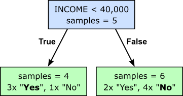
If we use this Decision Stump to classify all training samples, we see that we make $3$ misclassifications:
- ID 4 gets misclassified as "Yes" since the majority of customers with an annual income less than $40k$ default on their credit.
- ID 3 and ID 10 get misclassified as "No" since the majority of customers with an annual income more than $40k$ will not default on their credit.
We can also show this outcome by color coding the data table with green rows reflecting correct classifications and red rows reflecting misclassification.
| Weight wi | ID | AGE | MARITAL_STATUS | ANNUAL_INCOME | DEFAULTED |
|---|---|---|---|---|---|
| 0.1 | 1 | 24 | Single | 28,000 | Yes |
| 0.1 | 2 | 45 | Married | 92,000 | No |
| 0.1 | 3 | 31 | Single | 55,000 | Yes |
| 0.1 | 4 | 52 | Divorced | 38,000 | No |
| 0.1 | 5 | 29 | Married | 120,000 | No |
| 0.1 | 6 | 41 | Widowed | 47,000 | No |
| 0.1 | 7 | 22 | Single | 21,000 | Yes |
| 0.1 | 8 | 36 | Married | 75,000 | No |
| 0.1 | 9 | 58 | Divorced | 33,000 | Yes |
| 0.1 | 10 | 27 | Single | 65,000 | Yes |
AdaBoost now computes several values needed to update the weights $w_i$. First, it computes the total error $\epsilon$ for the weak learner as the sum of the current weights of all the misclassified samples. With $3$ misclassifications and all initial weights being $0.1$, we get a total error of $\epsilon = 0.3$. Next, based on the total error, AdaBoost computes the so-called "amount of say" $\alpha$ which measures how much influence a weak learner has on the final ensemble prediction. Weak learners that make fewer mistakes receive a larger amount of say, while learners that perform poorly receive a smaller amount of say. For a binary classification task — which we have here — the amount of say for a weak learner is computed as:
Plugging in the total error of $0.3$ we get an amount of say for this weak learner of $\alpha = 0.42$. Based on $\alpha$, AdaBoost now updates the weights of all samples. More specifically, AdaBoost reduces the weight of correctly classified samples, and increases the weight of wrongly classified samples using the following update rule:
This update rule does generally not result in new weights that will sum up to $1$. However, since this is required for AdaBoost to perform correctly, the last step is therefore to normalize all weights using $w_{i} = w_i/\sum_{i}^{N}w_i$. Thus, after all these steps, we get the new weights for all data samples as shown in the table below (note that the weights do not exactly sum up to $1$ due to limited precision).
| Weight wi | ID | AGE | MARITAL_STATUS | ANNUAL_INCOME | DEFAULTED |
|---|---|---|---|---|---|
| 0.071 | 1 | 24 | Single | 28,000 | Yes |
| 0.071 | 2 | 45 | Married | 92,000 | No |
| 0.167 | 3 | 31 | Single | 55,000 | Yes |
| 0.167 | 4 | 52 | Divorced | 38,000 | No |
| 0.071 | 5 | 29 | Married | 120,000 | No |
| 0.071 | 6 | 41 | Widowed | 47,000 | No |
| 0.071 | 7 | 22 | Single | 21,000 | Yes |
| 0.071 | 8 | 36 | Married | 75,000 | No |
| 0.071 | 9 | 58 | Divorced | 33,000 | Yes |
| 0.167 | 10 | 27 | Single | 65,000 | Yes |
Notice how the weights of misclassified samples increased, and the weights of correctly classified samples decreased. The whole idea of AdaBoost is to use these weights in such a way that subsequent learners pay more attention to misclassification to improve on the errors of previous learners. How this is done in detail will be covered in the next section.
Incorporating Weights
So far, we have seen how AdaBoost uses the accuracy of a learn in terms of its misclassification to update the weights, i.e., increasing the weights of misclassified samples and decreasing the weights of correctly classified samples. However, we still need to address how the weights actually affect the training process. Recall that the general idea behind AdaBoost — and boosting in general — is that subsequent learners pay more attention to "bad" samples, that is, samples that have been (frequently) misclassified. Now that we have a way to identify bad samples using the sample weights, we now need a way to formalize the idea of learners to "pay more attention" to bad samples. There are two fundamental approaches for this: incorporate the weights into the loss or generated bootstrap samples based on the sample weights.
Weighted Loss
When training a supervised machine learning model, the loss function is the means to quantify how good or bad the current model is performing. Normally, each training sample contributes equally to the total loss. Thus, assuming $N$ training samples, each sample contributes $1/N$ to the total loss. In contrast, in a weighted setup such as AdaBoost, each data point $i$ is assigned an individual weight vector, $w_i$, and the loss function is modified so that the penalty for misclassifying point $i$ is multiplied by $w_i$:
where $\mathcal{L}(y_i, \hat{y}_i)$ is the sample loss quantifying the loss by computing the difference between the predicted value and the ground truth value of the $i$-th sample (e.g., the Mean Sqared Error (MSE) for regression tasks or the Cross-Entropy loss for classification tasks).
When training an AdaBoost ensemble model with Decision Trees as base learners, the weighted loss is incorporated at the most fundamental level of the tree's construction: the splitting criterion (such as Gini Impurity or Entropy). Instead of just counting the number of misclassified samples to determine the best split, the decision tree calculates the sum of the weights of the samples. In other words, misclassified samples with a higher sample weight have more impact on finding the best split of a current node in the tree.
For example, for classification task with $C$ classes, the Gini score (or Gini impurity) computes the probabilities $P(c\mid t)$ that a class $c\in C$ appears in node $t$ as the relative frequency of seeing class $c$ in node $t$:
Instead of using the raw counts, AdaBoost computes the weighted probability as:
Because $P(c\mid t)$ is now dominated by the weights rather than the raw count of samples, any data point with a massive weight (a mistake from the previous round) will heavily skew $P(c\mid t)$ toward its own class. This, in turn will affect the final Gini score of a node $t$, which is computed as $Gini(t) = 1 - \sum_{c\in C} P(c|t)^2$. In simple terms, the process of finding the best split of a node in a Decision Tree is now determined by the sample weights. In practice, this typically manifests as:
- isolating high-weight samples in their own leaf node,
- creating a branch that captures a cluster of difficult samples,
- choosing a threshold specifically because it separates a group of high-weight samples from the rest.
So a useful way to think about it is:
Summing up, in ordinary Decision Trees, the split criterion tries to improve purity for as many samples as possible. In AdaBoost, the split criterion tries to improve purity for as much weight as possible.
Weighted Resampling
An alternative to modifying the Decision Tree learning algorithm to directly incorporate sample weights into the split criterion is to leave the tree induction process unchanged and instead use the sample weights during data sampling. In this approach, a bootstrap sample is generated by drawing training samples with replacement according to their weights, such that samples with higher weights have a greater probability of being selected multiple times, while samples with lower weights are selected less frequently or may not be selected at all. The resulting bootstrap dataset is then used to train a standard decision tree without any modifications to its impurity measures or split selection procedure. This strategy allows existing tree learning implementations to be reused while still ensuring that the boosting algorithm emphasizes difficult-to-classify samples, since high-weight samples are more likely to appear in the training data presented to subsequent weak learners.
To give an example, let's go back to our example dataset after we updated the weights as a result from training the first learner — where nothing exciting happened since all sample weights initially were the same.
| Weight wi | ID | AGE | MARITAL_STATUS | ANNUAL_INCOME | DEFAULTED |
|---|---|---|---|---|---|
| 0.071 | 1 | 24 | Single | 28,000 | Yes |
| 0.071 | 2 | 45 | Married | 92,000 | No |
| 0.167 | 3 | 31 | Single | 55,000 | Yes |
| 0.167 | 4 | 52 | Divorced | 38,000 | No |
| 0.071 | 5 | 29 | Married | 120,000 | No |
| 0.071 | 6 | 41 | Widowed | 47,000 | No |
| 0.071 | 7 | 22 | Single | 21,000 | Yes |
| 0.071 | 8 | 36 | Married | 75,000 | No |
| 0.071 | 9 | 58 | Divorced | 33,000 | Yes |
| 0.167 | 10 | 27 | Single | 65,000 | Yes |
Now, instead of directly training the next learner on this dataset, we create a bootstrap sample of the same size by sampling the original dataset. The sampling is random but probabilities are proportional to the weights, meaning a sample with a high(er) weight is more likely to be picked than a sample with a low(er) weight. Since we sample with replacement, an individual sample may appear multiple times or not at all in the bootstrap sample. For example, a bootstrap sample for our example dataset might look as follows:
| Weight wi | ID | AGE | MARITAL_STATUS | ANNUAL_INCOME | DEFAULTED |
|---|---|---|---|---|---|
| 0.071 | 1 | 24 | Single | 28,000 | Yes |
| 0.167 | 3 | 31 | Single | 55,000 | Yes |
| 0.167 | 3 | 31 | Single | 55,000 | Yes |
| 0.167 | 4 | 52 | Divorced | 38,000 | No |
| 0.071 | 5 | 29 | Married | 120,000 | No |
| 0.071 | 6 | 41 | Widowed | 47,000 | No |
| 0.071 | 9 | 58 | Divorced | 33,000 | Yes |
| 0.167 | 10 | 27 | Single | 65,000 | Yes |
| 0.167 | 10 | 27 | Single | 65,000 | Yes |
| 0.167 | 10 | 27 | Single | 65,000 | Yes |
Here, ID 3 was picked twice and ID 10 was picked three times since their higher weight made them more likely part of the bootstrap sample. Based on this bootstrap sample, the next learner is not trained, which again results in a Decision Stump, new misclassifications and therefore new weights. Two important details are worth mentioning:
- Each bootstrap sample is generated by drawing from the original dataset (not the previous bootstrap sample).
- The misclassified samples of each learner (i.e., Decision stump) are derived using the original data — that is, we use the bootstrap sample only to train the learner, but we evaluate it using the original dataset, this includes that we always update the weights in the original dataset.
Weighted loss vs. weighted resampling. It is important to point out that these two approaches are not equivalent. Based on the formula for the weighted probability $P(c\mid t)$ we can see that, for example, a sample with weight $w_i = 0.2$ always contributes twice as much as a sample with weight $w_j = 0.1$ during the split search. The influence of the weights is exact and deterministic. In contrast, weighted sampling has a nondeterministic component, meaning that the weights influence the tree only indirectly through the composition of the training sample. For example, a bootstrap sample may look like the original dataset (or other previous bootstrap sample) even though the sample's weights have changed (a lot). A low probability does not mean a zero probability. A useful way to think about it is:
- Weighted Loss: "Treat this observation as if it were worth 10 ordinary observations."
- Weighted resampling: "I will probably show you this observation about 10 times as often as a normal observation."
If the dataset is large and many bootstrap samples are considered, these viewpoints become similar. For a single tree, however, the weighted loss approach is more precise and typically produces lower-variance behavior. It is therefore the default approach of existing implementations. Note that this assumes that the implementation of the base learner requires to support sample weights. For example the DecisionTreeClassifier class, but also other model implementations, of the scikit-learn support sample weights out of the box. This makes implementing AdaBoost on top of these base learner classes quite straightforward. Of course, in practice, you are likely to directly use the AdaBoostClassifier or AdaBoostRegressor classes when already working with scikit-learn.
Making Predictions
AdaBoost trains multiple base learners (e.g., Decision Stump), with each subsequent learner focusing on the errors of the previous one; the number of learners is a hyperparameter, say, $K$. This means that after the training, our model consists of $K$ Decision Stumps. To use this model to make predictions, the most important observation is that the different Decision Trees will generally have performed differently with respect to the total error $\epsilon$; note that this includes the training error of each subsequent weak learner does not necessarily go down, and may even go up. Thus, we cannot make predictions based on, for example, a simple majority voting scheme (like in Random Forests).
During inference, we need to take the training accuracy of each weak learner into account. In AdaBoost, this is reflected by the "amount of say" $\alpha$. Recall that a high $\alpha$ value shows that the learner made very few mistakes, and vice versa for low $\alpha$ values. In the case of regression tasks, the final prediction derives from the weighted sum of outputs from all learners, with the weights being the respective $\alpha$ values. If $f_t$ denotes the of $m$-th weak learner, the final prediction is:
For classification tasks, we also give the input to all $t$ weak learners to get $t$ labels. However, instead of going with the majority label, we return the class with the highest amount of say. To illustrate this, assume that we trained an AdaBoost model based on $8$ Decision Stumps $f_1$, $f_2$, ..., $f_8$ on our example dataset (binary classification). During the training, we have computed for each weak learner its amount of say $\alpha_t$. Now let's assume that for a new data sample $x$, the learners $f_1$, $f_3$, and $f_8$ predict "Yes", while all other learners predict "No". The table below presents all the required information.
| Amount of Say | Output | |
|---|---|---|
| $f_1$ | $\alpha_1 = 0.34 $ | $f_1(x)$ = "Yes" |
| $f_2$ | $\alpha_2 = 0.14 $ | $f_2(x)$ = "No" |
| $f_3$ | $\alpha_3 = 1.20 $ | $f_3(x)$ = "Yes" |
| $f_4$ | $\alpha_4 = 0.58$ | $f_4(x)$ = "No" |
| $f_5$ | $\alpha_5 = 0.09$ | $f_5(x)$ = "No" |
| $f_6$ | $\alpha_6 = 0.62$ | $f_6(x)$ = "No" |
| $f_7$ | $\alpha_7 = 0.45$ | $f_7(x)$ = "No" |
| $f_8$ | $\alpha_8 = 0.97$ | $f_8(x)$ = "Yes" |
Since learners $f_1$, $f_3$, and $f_8$ have predicted "Yes", we need to sum $\alpha_1 + \alpha_2 + \alpha_8 = 2.51$ to get the overall amount of say for "Yes". Summing up the remaining $\alpha$ values for all learners that have predicted "No", we get an overall amount of say of $1.88$. This means that, even though the majority of learners predicted "No", the overall amount of say for "Yes" is larger, making this the final prediction.
Notice that during inference, AdaBoost supports the parallelization of the individual learners, even though the training was strictly sequential. This is different compared to the idea of gradient boosting, as we discuss in a moment.
Summary (AdaBoost). AdaBoost improves predictive performance by iteratively focusing on the training samples that are hardest to predict. It does this by assigning a weight to each training sample, where samples that are consistently classified correctly are considered "easy" and receive lower weights, while misclassified or difficult samples receive higher weights. These sample weights are then incorporated into the training process of each subsequent weak learner, causing the learner to pay more attention to difficult cases and less attention to easy ones. By repeatedly reweighting the samples and combining the resulting weak learners into a weighted ensemble, AdaBoost gradually builds a strong predictor that performs well across the entire dataset.
Predicting the Residuals (Gradient Boosting)
AdaBoost improves an ensemble by reweighting the training samples, forcing each new learner to focus more on the examples that previous learners found difficult. An alternative approach is gradient boosting, which shifts the focus from the samples themselves to the errors made by the current ensemble. Instead of increasing the weights of misclassified or poorly predicted observations, each new (weak) learner is trained to predict the residuals — the differences between the observed values and the ensemble's current predictions. By repeatedly fitting learners to these residuals and adding their predictions to the ensemble, gradient boosting gradually reduces the overall prediction error and builds an increasingly accurate model, i.e., a strong learner.
Gradient boosting is a family of ensemble learning algorithms that build models by sequentially fitting learners to the errors made by the current ensemble. The most basic member of this family is the Gradient Boosted Machine (GBM), while XGBoost, LightGBM, and CatBoost are advanced extensions that introduce improvements in predictive performance, computational efficiency, scalability, and support for specific data types such as categorical features. Despite their differences, all of these algorithms typically use Decision Trees as their base learners, combining many weak trees into a powerful predictive model.
Gradient Boosting Machine (GBM)
Gradient Boosted Machines (GBMs) are an ensemble learning method that builds a strong predictive model by sequentially combining many weak learners, typically decision trees. The process begins with an initial prediction for every training sample, such as the mean target value in regression problems. The residuals, which represent the errors of the current model, are then computed as the difference between the ground-truth values and the model's predictions. A new learner is trained specifically to predict these residuals, thereby focusing on the mistakes made by the existing ensemble.
Once the learner has been trained, its predicted residuals are added to the current predictions, often scaled by a learning rate to control the magnitude of the update. This adjustment reduces the remaining prediction error and improves the model's overall accuracy. The cycle of computing residuals, training a new learner, and updating predictions is repeated iteratively, with each learner correcting the errors of its predecessors. Training continues until a predefined number of learners has been added or another stopping criterion is reached, resulting in a powerful ensemble model that progressively refines its predictions.
Training GBMs
Let's use a simple example to illustrate the idea, again using our example dataset of bank customers. Since the computation of residuals is more straightforward for numerical values, we now consider a regression task where the goal is to predict a customer's credit limit in dollars. The table below shows the dataset with all $N=10$ samples.
| ID | AGE | MARITAL_STATUS | ANNUAL_INCOME | LIMIT |
|---|---|---|---|---|
| 1 | 24 | Single | 28,000 | 1,000 |
| 2 | 45 | Married | 92,000 | 1,200 |
| 3 | 31 | Single | 55,000 | 1,400 |
| 4 | 52 | Divorced | 38,000 | 900 |
| 5 | 29 | Married | 120,000 | 1,000 |
| 6 | 41 | Widowed | 47,000 | 600 |
| 7 | 22 | Single | 21,000 | 900 |
| 8 | 36 | Married | 75,000 | 1,100 |
| 9 | 58 | Divorced | 33,000 | 600 |
| 10 | 27 | Single | 65,000 | 1,300 |
For regression tasks, the initial prediction of a Gradient Boosted Machine can, in principle, be any constant value. However, because no information from the features has been incorporated at the start of training, a sensible default is to predict the mean of all target values in the training data. This choice minimizes the overall squared error among all possible constant predictions and therefore provides the best baseline estimate before any learners are trained. Starting from the mean ensures that the subsequent learners focus on explaining the remaining variation in the data by predicting the residuals, which are the differences between the observed outcomes and the current predictions.
For our example dataset, the mean of all target values (i.e. feature LIMIT) is conveniently $1,000$. Thus, if $F_{0}$ denotes our initial model, we have $F_{0}(\mathbf{x}_i) = 1,000$ as the initial prediction for all training samples. For the first learner , we then need to compute the residual $r_{i}^{(1)}$ for a data sample $\mathbf{x}_i$ as the difference between its ground truth $y_i$ and the current prediction; more formally $r_{i}^{(1)} = y_i - F_{0}(\mathbf{x}_i)$. For example, the last sample $\mathbf{x}_{10}$ has a ground truth values of $y_{10} = 1,300$, meaning that after subtracting the initial prediction $F_{0}(\mathbf{x}_{10}) = 1,000$, we get its residual $r_{10}^{(1)} = 300$. The updated table below shows the result after performing this step for all data samples.
| ID | AGE | MARITAL_STATUS | ANNUAL_INCOME | LIMIT $y_i$ | $F_{0}(\mathbf{x}_i)$ | $r_{i}^{(1)}$ |
|---|---|---|---|---|---|---|
| 1 | 24 | Single | 28,000 | 1,000 | 1,000 | 0 |
| 2 | 45 | Married | 92,000 | 1,200 | 1,000 | 200 |
| 3 | 31 | Single | 55,000 | 1,400 | 1,000 | 300 |
| 4 | 52 | Divorced | 38,000 | 900 | 1,000 | -100 |
| 5 | 29 | Married | 120,000 | 1,000 | 1,000 | 0 |
| 6 | 41 | Widowed | 47,000 | 600 | 1,000 | -400 |
| 7 | 22 | Single | 21,000 | 900 | 1,000 | -100 |
| 8 | 36 | Married | 75,000 | 1,100 | 1,000 | 100 |
| 9 | 58 | Divorced | 33,000 | 600 | 1,000 | -400 |
| 10 | 27 | Single | 65,000 | 1,300 | 1,000 | 300 |
The GBM now trains the first learner $f_1$ with the task to predict the residuals $f_1(\mathbf{x}_i)$ for each training sample $\mathbf{x}_i$. As commonly done, we rely on Decision Trees — more specifically, Decision Stumps since we train weak learners — as the base learner. To keep the example simple and illustrative, let's assume we have trained a Decision Stump with a maximum depth of $2$ and which only considered the feature ANNUAL_INCOME to. Again, this limitation is only to ensure convenient results for the running example. With these consideration, the resulting Decision Stump looks as follows:
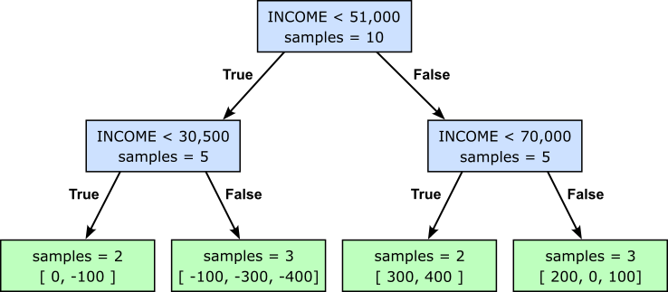
In the next step, we use the learner $f_1$ to predict the target values for each data sample. Keep in mind that our learner is a shallow tree (i.e., a Decision Stump), so its predictions are generally the means of all the values within the respective child node. For example, the right-most leaf node contains the residuals for the 2nd, 5th, and 8th sample. The mean of these three residuals is $(200+0+100)/3 = 100$. This means that the prediction for these three sample with respect to learner $f_1$ are $f_1(\mathbf{x}_2) = f_1(\mathbf{x}_5) = f_1(\mathbf{x}_8) = 100$. The table below includes the predicted values for all data samples.
| ID | AGE | MARITAL_STATUS | ANNUAL_INCOME | LIMIT $y_i$ | $F_{0}(\mathbf{x}_i)$ | $r_{i}^{(1)}$ | $f_1(\mathbf{x}_i)$ |
|---|---|---|---|---|---|---|---|
| 1 | 24 | Single | 28,000 | 1,000 | 1,000 | 0 | -50 |
| 2 | 45 | Married | 92,000 | 1,200 | 1,000 | 200 | 100 |
| 3 | 31 | Single | 55,000 | 1,400 | 1,000 | 400 | 350 |
| 4 | 52 | Divorced | 38,000 | 900 | 1,000 | -100 | -300 |
| 5 | 29 | Married | 120,000 | 1,000 | 1,000 | 0 | 100 |
| 6 | 41 | Widowed | 47,000 | 600 | 1,000 | -400 | -300 |
| 7 | 22 | Single | 21,000 | 900 | 1,000 | -100 | -50 |
| 8 | 36 | Married | 75,000 | 1,100 | 1,000 | 100 | 100 |
| 9 | 58 | Divorced | 33,000 | 600 | 1,000 | -400 | -300 |
| 10 | 27 | Single | 65,000 | 1,300 | 1,000 | 300 | 350 |
The last step — well, for this first iteration — is to update our current $F_{0}$ with respect to the predicted residual $f_1(\mathbf{x}_i)$. In general, although this is not guaranteed, samples with current predictions larger than their ground truth values will have positive predicted residuals — recall that we compute $r_{i}^{(1)} = y_i - F_{0}(\mathbf{x}_i)$. As such, to get the current prediction closer to the ground truth, we need to add the current prediction and the residuals, i.e., $F_{1}(\mathbf{x}_i) = F_{0}(\mathbf{x}_i) + f_1(\mathbf{x}_i)$.
However, using the raw predicted residuals would typically cause the learner to make (overly) large corrections. As a result, the ensemble may fit the training data too aggressively, including noise and random fluctuations, which increases the risk of overfitting and poor performance on unseen data. In practice, the model can become unstable, with later learners overcorrecting errors made by previous learners rather than gradually refining the predictions. Thus, instead of adding the raw prediction residuals, GBM introduces a learning rate $\eta$ to scale down the predicted residuals. This gives us the final update rule: $F_{1}(\mathbf{x}_i) = F_{0}(\mathbf{x}_i) + \eta f_1(\mathbf{x}_i)$. Setting $\eta = 0.1$ and applying the rules to our data we get:
| ID | AGE | MARITAL_STATUS | ANNUAL_INCOME | LIMIT $y_i$ | $F_{0}(\mathbf{x}_i)$ | $r_{i}^{(1)}$ | $f_1(\mathbf{x}_i)$ | $F_{1}(\mathbf{x}_i)$ |
|---|---|---|---|---|---|---|---|---|
| 1 | 24 | Single | 28,000 | 1,000 | 1,000 | 0 | -50 | 995 |
| 2 | 45 | Married | 92,000 | 1,200 | 1,000 | 200 | 100 | 1,010 |
| 3 | 31 | Single | 55,000 | 1,400 | 1,000 | 400 | 350 | 1,035 |
| 4 | 52 | Divorced | 38,000 | 900 | 1,000 | -100 | -300 | 970 |
| 5 | 29 | Married | 120,000 | 1,000 | 1,000 | 0 | 100 | 1,010 |
| 6 | 41 | Widowed | 47,000 | 600 | 1,000 | -400 | -300 | 970 |
| 7 | 22 | Single | 21,000 | 900 | 1,000 | -100 | -50 | 995 |
| 8 | 36 | Married | 75,000 | 1,100 | 1,000 | 100 | 100 | 1010 |
| 9 | 58 | Divorced | 33,000 | 600 | 1,000 | -400 | -300 | 970 |
| 10 | 27 | Single | 65,000 | 1,300 | 1,000 | 300 | 350 | 1,035 |
With updating the current prediction, we have completed the first iteration and can now continue with the next iterations using the updated predictions as the starting point; of course, the core steps remain exactly the same. In general, in the $m$-th iteration, we perform the following steps:
- Compute the residuals: $\ r_{i}^{(m)} = y_i - F_{m-1}(\mathbf{x}_i)$
- Fit a weak learner $\ f_m \ $ on residuals
- Compute the predicted residuals $\ f_m(\mathbf{x}_i)$
- Update the current predictions: $\ F_{m}(\mathbf{x}_i) = F_{m-1}(\mathbf{x}_i) + \eta f_m(\mathbf{x}_i)$
To add to our example, the table below shows the results after the second iteration.
| ID | AGE | MARITAL_STATUS | ANNUAL_INCOME | LIMIT $y_i$ | $F_{0}(\mathbf{x}_i)$ | $r_{i}^{(1)}$ | $f_1(\mathbf{x}_i)$ | $F_{1}(\mathbf{x}_i)$ | $r_{i}^{(2)}$ | $f_2(\mathbf{x}_i)$ | $F_{2}(\mathbf{x}_i)$ |
|---|---|---|---|---|---|---|---|---|---|---|---|
| 1 | 24 | Single | 28,000 | 1,000 | 1,000 | 0 | -50 | 995 | 5 | -45 | 990.5 |
| 2 | 45 | Married | 92,000 | 1,200 | 1,000 | 200 | 100 | 1,010 | 190 | 90 | 1019.0 |
| 3 | 31 | Single | 55,000 | 1,400 | 1,000 | 400 | 350 | 1,035 | 365 | 315 | 1066.5 |
| 4 | 52 | Divorced | 38,000 | 900 | 1,000 | -100 | -300 | 970 | -70 | -270 | 943.0 |
| 5 | 29 | Married | 120,000 | 1,000 | 1,000 | 0 | 100 | 1,010 | -10 | 90 | 1019.0 |
| 6 | 41 | Widowed | 47,000 | 600 | 1,000 | -400 | -300 | 970 | -370 | -270 | 943.0 |
| 7 | 22 | Single | 21,000 | 900 | 1,000 | -100 | -50 | 995 | -95 | -45 | 990.5 |
| 8 | 36 | Married | 75,000 | 1,100 | 1,000 | 100 | 100 | 1010 | 90 | 90 | 1019.0 |
| 9 | 58 | Divorced | 33,000 | 600 | 1,000 | -400 | -300 | 970 | -370 | -270 | 943.0 |
| 10 | 27 | Single | 65,000 | 1,300 | 1,000 | 300 | 350 | 1,035 | 265 | 315 | 1066.5 |
This process continues until the specified number of learners have been trained; the number of learners is a hyperparameter, and so is the learning rate $\eta$. Keep in mind that getting the predicted residuals $f_m(\mathbf{x}_i)$ requires fitting a learner $f_m$ to the residuals $r_{i}^{(m)}$. The long-term trend of this sequential training of learners is:
- The residual $r_{i}^{(m)}$ will go towards $0$
- The predictions $F_{m}(\mathbf{x}_i)$ will get closer to the true values $y_i$
Important: Note that this behavior describes the long-term trend. Both the residuals and the difference between predictions and true values are generally monotonically decreasing. To give an example, which you may have already spotted, the initial prediction of the first sample already matches the true values of $1,000$. However, the update using the predicted residuals — which is generally the mean of several residuals — causes the prediction to actually deviate from the true value at first.
Like with any boosting strategy, the final output of training a GBM is a sequence of trained based learners $f_1$, $f_2$, ..., $f_K$, typically Decision Stumps, with $K$ being the specified number of learners.
Making Predictions
Once a Gradient Boosted Machine has been trained, it makes predictions by following the same sequence of updates that was learned during training. For a new sample $\mathbf{x}$, the prediction is initialized with the same constant value used at the start of training (e.g., $F_{0}(\mathbf{x}_i) = 1,000$ for our running example). The sample is then passed through the first weak learner $f_1$, whose output $f_1(\mathbf{x}_i)$ is added to the current prediction, scaled by the learning rate $\eta$. This process is repeated sequentially for all trained learners in the ensemble. Each learner contributes a small correction to the current prediction, gradually refining it based on patterns it learned from the residuals during training. Mathematically, the prediction $\hat{y}_{i}$ for an unseen sample $\mathbf{x}_i$ is computed as:
Note that, compared to AdaBoost, inference in GBMs is also strictly sequential (not just the training). This is because each learner in a GBM predicts a correction to the current prediction, making the output of one learner a necessary input for the next. Consequently, the learners cannot be evaluated independently and combined afterward; instead, predictions must be updated step by step by traversing the entire sequence of trained learners in order.
GBMs for Classification
To outline the idea and the basic steps of Gradient Boosted Machines, we used an example dataset for a regression task to cover the initialization as well as the first two iterations to provide a complete worked example. We chose a regression task since the notions of initial/current predictions as well as of residuals are much more straightforward when dealing with numerical target values (here: dollar values). However, GBMs also support classification tasks, and all the core steps remain exactly the same. While an in-depth discussion is beyond this overview notebook, here are the basic requirements for training a GBM for classification task assuming $C$ different classes:
Initial/current predictions: For each sample, the model GBM starts with a score (e.g., logits or probabilities) for each class, representing the prior belief about the probability of each class before considering any features. For example, assuming a balanced dataset with $4$ classes and using probabilities as scores, each sample will start with an initial prediction $(0.25, 0.25, 0.25, 0.25)$, i.e., a probability of $0.25$ for each class.
Computing residuals: Like before the residuals are computed as the difference between the true values and the current predictions. Again, assuming a classification task with $C=4$, a target vector of $(0, 1, 0, 0)$ for a training sample $\mathbf{x}_i$ indicates that $\mathbf{x}_i$ belongs to Class $2$. Computing the residuals now comes down to subtracting the target vector for the current predictions vector, for example:
Predicting residual: Computing the predicted residuals using the trained learner. Since the residuals are numerical values (and not class labels), the learner will in fact be a regression model (e.g., a Decision Stump regressor as used above). More specifically, given $C$ classes, a GBM will train $C$ regression models in each iteration, one for each class — although alternatives multi-output regression trees are possible. On learner with its $C$ regression models is trained, we use the learner to predict the residual for each training sample. Like before, since the trees are very shallow, the predicted residuals are likely to be the means across several samples. For example, for our training sample $\mathbf{x}_i$ might get the vector of predicted residuals $f_1(\mathbf{x}_i) = (-0.50, 0.70, -0.40, -0.60)$.
Updating model: Using the predicted residual to update the current prediction is done using the same rule: $ F_{m}(\mathbf{x}_i) = F_{m-1}(\mathbf{x}_i) + \eta f_m(\mathbf{x}_i)$. For our example, we can now update the current predictions vector $\hat{y}_{i}^{(1)}$ using the vector of prediction residuals $f_1(\mathbf{x}_i)$, and get:
In short, GBMs and variants/extensions such as XGBoost, LightGBM, and CatBoost, work internally very similarly: they use regression trees regardless of whether the final task is regression or classification. The difference lies not in the type of tree being trained, but in the loss function being optimized and how the residuals are computed. A useful way to think about gradient boosting is:
- GBM for regression: regression trees predict residuals of the target value.
- GBM for classification: regression trees predict residuals of the classification loss.
The main take-away message is that in both cases, the base learners are fundamentally performing regression.
Where is the Gradient?
The name Gradient Boosted Machines originates from the idea that each newly trained learner attempts to move the model in a direction that reduces the prediction error. Recall that for both regression and classification tasks, GBM always trains regression models for its learners, since the targets are always numerical values; see above. The standard loss $\mathcal{L}(y_i, \hat{y}_i)$ for a single sample $\mathbf{x}_i$ regression task is the squared error. However, keep in mind that we need to compute this loss each learner $f_m$, which is defined as:
where $\hat{y}_i^{(m)} = F_{m}(\mathbf{x}_i)$, i.e., the output of the model after $m$ iterations. The factor $1/2$ is not important, but it makes the final result more convenient, as we see in a moment. We can no compute the gradient $g_i^{(m)}$ for sample $\mathbf{x}_i$ by computing the first derivative of the loss with respect to the predicted output (here: the predicted residual):
Here we can see the convenience of factor $1/2$. Since we want to reduce the loss, we move in the direction of the negative gradient. We get the negative gradient by multiplying both sides by $-1$, which gives us $y_i - y_i^{(m)}$, which is simply our expression to compute $r_{i}^{(m)}$. This is why the residuals in a regression GBM can be interpreted as the negative gradients of the squared-error loss. Historically, early explanations of boosting often described the algorithm as "fitting the residuals". The more general gradient boosting framework recognizes that what is actually being fitted is the negative gradient of the loss function. For squared-error loss, these two concepts happen to be identical:
Side notes. While the connection between the gradient and the residuals seem rather straightforward, there are some details worth pointing out:
The term gradient is somewhat of a misnomer in the simplified residual-based view of GBMs. In calculus, a gradient describes a continuous rate of change, whereas GBMs update their predictions through a sequence of discrete steps, each represented by a newly trained weak learner. The residuals can therefore be viewed as an approximation of the direction in which the model should move to reduce the error, rather than a true gradient in the mathematical sense. This interpretation becomes more accurate in the general formulation of gradient boosting, where learners are fitted to the negative gradient of a chosen loss function, but the updates themselves remain discrete additions of weak learners.
To be more technically correct, $r_{i}^{(m)}$ is called the pseudo-residual because $r_{i}^{(m)}$ is only the true residual $y_i - \hat{y}_i^{(m)}$ for the squared error loss. This changes for different loss / error functions. For example, if we would use the absolute error (L1 loss) where $\mathcal{L}^{(0)} = |y_i - \hat{y}_i^{(0)}|$ to be more robust against outliers, the negative gradient changes to:
Summary. Gradient Boosted Machines (GBMs) are based on the fundamental idea of building a strong predictive model by sequentially combining many weak learners, typically decision trees. Starting from an initial prediction, each learner is trained to correct the errors of the current model by predicting residuals or, more generally, the negative gradients of a chosen loss function. The predictions are then updated iteratively, allowing the ensemble to gradually improve its performance. This stage-wise learning process enables GBMs to model complex relationships while maintaining relatively simple individual learners.
This core boosting principle forms the foundation of many modern gradient boosting frameworks, including XGBoost, LightGBM, and CatBoost. While these frameworks introduce additional innovations such as second-order optimization, regularization, specialized handling of categorical features, improved treatment of missing values, and highly optimized training procedures, they all retain the central idea of iteratively adding learners that reduce the remaining prediction error. As a result, understanding the basic mechanics of GBMs provides the conceptual basis for understanding these more advanced and widely used boosting algorithms.
XGBoost
XGBoost (eXtreme Gradient Boosting) is one of the most popular and widely used boosting frameworks in machine learning. It builds upon the fundamental ideas of Gradient Boosted Machines (GBMs), which iteratively train weak learners to correct the errors of the current model, while introducing several enhancements that improve both predictive performance and computational efficiency. As a result, XGBoost has become a standard choice for many machine-learning competitions and real-world applications, particularly for structured tabular data.
The two most important extensions introduced by XGBoost are the use of Newton's method and regularization. While traditional GBMs rely only on first-order gradient information, XGBoost additionally incorporates second-order derivative information, allowing it to make more informed optimization steps and often converge faster. Furthermore, XGBoost explicitly regularizes the complexity of the learned trees, helping to reduce overfitting and improve generalization. Beyond these core innovations, XGBoost includes numerous practical improvements, such as automatic handling of missing values, row and feature subsampling, tree pruning, and a highly optimized implementation that enables efficient training on large datasets. Together, these enhancements make XGBoost both more powerful and more scalable than traditional GBMs.
The following sections aim to provide the intuition and explain the basic concepts behind these improvements that XGBoost makes to GBMs; again, a deep dive into XGBoost is beyond the scope of this overview notebook.
Newton Boosting
We just saw how GBMs use the first-order derivative (i.e., the gradients) to find the residuals (i.e., the direction of the error). Using only the first-order derivative (the gradient) provides information about the direction in which the loss function is increasing or decreasing, but it does not indicate how quickly the slope itself is changing. As a result, optimization steps may be too large in regions where the loss function is steep or too small in flatter regions, leading to slower convergence or less accurate updates.
XGBoost uses Newton Boosting, which itself is based on Newton's method, a general optimization algorithm that uses both the first and second derivatives of a function to find a minimum or maximum. Newton Boosting applies the idea of Newton's method within the gradient boosting framework. Instead of fitting learners to the negative gradient alone (as in traditional gradient boosting), it uses both the gradient and Hessian (second derivative) information when training the learners. The second-order derivative captures the curvature of the loss function and therefore provides information about the local shape of the optimization landscape. By incorporating both the gradient and the curvature, Newton's method can estimate not only the direction but also the appropriate magnitude of an update, allowing XGBoost to make more effective optimization steps and often converge faster than methods based solely on first-order information.
Let's see how this looks like for the squared error loss $\mathcal{L}(y_i, \hat{y}_i) = \frac{1}{2}\left(y_i -\hat{y}_i \right)^2$ for a training sample $\mathbf{x}_i$. Well already know that the negative gradient $-g_i$ for $\mathbf{x}_i$ is:
Now, the second-order derivative, or the Hessian $h_i$, for sample $\mathbf{x}_i$ is defined as
In short, for the standard squared error loss, the Hessian is simply $h_i = 1$, meaning that every training sample contributes equally to the second-order information used by XGBoost. However, for other loss functions the Hessian may vary from sample to sample and depends on the current prediction. In these cases, the Hessian provides additional information about the local curvature of the loss function, allowing XGBoost to adapt the magnitude of its updates based on how sensitive the loss is to changes in the predictions.
Recall that each boosting iteration first requires to compute the residual (or rather the pseudo-residual). XGBoost is computing the residuals exactly as traditional GBMs: the difference between the current predictions and the true values. In other words, for computing the residuals, XGBoost uses only the gradient $g_i$ (i.e., the first-order derivative information). So far, XGBoost and GBMs behave the same. The Hessian $h_i$ (i.e., the second-order derivative information) is used for training the learner and computing the predicted residual. To show how this works, we first need to talk about regularization, the other core concept the XGBoost introduces to GBMs.
Regularization
Regularization is a technique used to reduce overfitting by discouraging overly complex models that fit not only the underlying patterns in the training data but also noise and random fluctuations. It does so by introducing a penalty for model complexity into the optimization objective, for example by limiting the magnitude of model parameters or the complexity of decision trees. As a result, regularization often improves a model's ability to generalize to unseen data, leading to better predictive performance in practice.
A basic GBM controls overfitting primarily through heuristics such as limiting tree depth (i.e., "manually" enforcing shallow trees through hyperparameters), tuning the learning rate $\eta$ (shrinkage), or subsampling data. In contrast, XGBoost explicitly integrates the concept of regularization — together with the gradient and Hessian information — into both the training and the prediction of residuals. Since these require some nontrivial extension to traditional GBMs, to focus here is to provide a basic intuition.
Let's start with the training. Recall when training a learner (i.e., Decision Tree/Stump) for a class GBM, the "only" goal is to minimize the overall loss $\mathcal{L} = \sum_{i=1}^{n} \mathcal{L}(y_i, \hat{y}_i)$, with $n$ being the total number of training samples. Trying to optimize this objective leads to the classic approach of finding the best splits using criteria such as the Mean Squared Error (MSE) or the Sum of Square Errors (SSE). Of course, optimizing this loss alone would result in strong learners and increase the risk of overfitting. This is why, when using GBMs, restricting the complexity of the trees using hyperparameters (e.g., the maximum depth of a tree, or the minimum number of samples to split a tree) is required.
In contrast, XGBoost uses regularization to automatically implement constraints on the complexity of the trained tree. The model does so by considering the following objective function:
where $\Omega(f_k)$ is the regularization term for the $k$-th tree in the sequence. For any tree $f$, this regularization term is defined as:
where:
- $T$ is the number of leaves in the tree
- $w_j$ is the prediction value stored in leaf $j$
- $\gamma$ is a penalty factor for each additional leaf
- $\lambda$ is the L2 regularization parameter
Intuitively, the first term $\gamma T$ discourages unnecessarily large trees by charging a cost for every leaf, and the second term $\frac{\lambda}{2}\sum_{j=1}^T w_j^2$ discourages extreme leaf predictions by shrinking leaf values toward zero. Regarding the latter, remember that we predict residuals, meaning that extreme predictions correspond to aggressive corrections when we update the current predictions — which we want to avoid to reduce the risk of overfitting! By penalizing large leaf values through the regularization term, XGBoost encourages the model to make more conservative updates.
Side note: Although XGBoost incorporates regularization to control model complexity and reduce overfitting, it still relies on hyperparameters such as the maximum tree depth, minimum child weight, and learning rate. Regularization penalizes overly complex trees, but it does not completely determine the structure of the model. Hyperparameters provide additional control over how the trees are grown and how aggressively the ensemble learns, allowing practitioners to balance predictive accuracy, computational efficiency, and generalization performance for a given dataset.
During a boosting iteration, at iteration $m$, when a new tree $f_m$ is added, the objective for this step is:
Directly optimizing XGBoost's objective function within a decision tree is mathematically challenging because the tree structure introduces discrete decisions, such as selecting split points and assigning observations to leaves. These decisions make the objective function non-differentiable and difficult to optimize analytically. To overcome this challenge, XGBoost approximates the loss function using a second-order Taylor expansion, transforming the original optimization problem into a simpler form that can be optimized efficiently when constructing the tree. Skipping the mathematical details here, equation for approximating the loss $\tilde{\mathcal{L}}^{(m)}$ is:
Firstly, notice that this approximation now incorporates both the gradient $g_i^{(1)}$ as well as the $f_i^{(m)}$, i.e., both first-order and second-order derivative information. More importantly, the mathematical convenience of the second-order Taylor expansion is that it transforms an arbitrary, potentially messy loss function into a clean, predictable quadratic expression in $f_t(\mathbf{x}_i)$. A quadratic function is the ultimate convenience tool in optimization because its properties are thoroughly understood and exceptionally easy to solve analytically.
Let's remind ourselves that $f_t(\mathbf{x}_i)$ is the predicted values for training sample $\mathbf{x}_i$, and this is the same value for all samples ending up in the same leaf of the $m$-th learner. Suppose a leaf $j$ predicts a constant value $w_j$ for all samples in that leaf, then $w_j = f_m(\mathbf{x_i})$ for all $\mathbf{x}_i$ where $i\in I_{j}$, and $I_j$ are the set of indices in leaf $j$. With that, we can express the $\tilde{\mathcal{L}}^{(m)}$ as the sum over the losses for all $T$ leaves. After some additional algebraic transformation, we get the following expression:
If we denote the sum of all gradients as $G_j^{(m)} = \sum_{i\in I_j} g_i^{{(m)}}$ and the sum of all Hessians as $H_j^{(m)} = \sum_{i\in I_j} h_i^{{(m)}}$, we can simplify the expresssion:
where $\mathcal{L}_j^{(m)}$ is the loss for leaf $j$.
Now, to optimize the approximated objective function, XGBoost must determine the best prediction value $w_j$ for each leaf. Since $w_j$ is the quantity that directly controls the leaf's contribution to the model's predictions, the objective can be viewed as a function of $w_j$. Taking the derivative with respect to $w_j$ measures how the objective changes when the leaf prediction is adjusted slightly. The optimal value of $w_j$ occurs at a minimum of the objective, where the slope is zero. Therefore, setting the derivative equal to zero allows XGBoost to find the leaf weight that minimizes the loss while accounting for regularization. Computing this derivatives gives us:
Note that all sum terms for leaves that are not leaf $j$ as well as the term $\gamma T$ do not depend on $w_j$ and are therefore considered constants when deriving the expression with respect to $w_j$. Setting the derivative to $0$ and solving for $w_j$ gives us the optimal value $w_i^{\ast}$:
Notice that the regularization parameter $\lambda$ is in the denominator. As $\lambda$ increases, the magnitude of $w_j$ shrinks toward zero. Intuitively, this makes the model more conservative by preventing individual leaves from making overly large corrections based on limited or noisy data. This is desirable because large leaf weights can lead to overfitting, where the model captures random fluctuations in the training data rather than genuine patterns.
Side note: Assuming the standard squared error with the Hessian $h_i^{(m)} = 1$, $H_j^{(m)}$ simplifies to $n_j^{(m)}$ being the number of samples in leaf $j$. Further, if we would set $\lambda = 0$, the expression for simplifies to the mean overall gradients $G_j^{(m)}$, which is exactly the value we get when using a traditional GBM.
We can now compute the minimal loss $\mathcal{L}_j^{(m)}$ for leaf $j$ by plugging the expression for $w_i^{\ast}$ back into the expression for $\mathcal{L}_j^{(m)}$:
By substituting the optimal leaf weight back into the approximated objective function, XGBoost obtains a measure of the contribution of each leaf to reduce the overall loss. This result can then be used to directly derive a splitting criterion that evaluates whether dividing a node into two child nodes leads to a sufficient improvement in model performance — which omit here to derive in full detail. During tree construction, candidate splits are compared based on the reduction in the objective function they achieve. Importantly, the splitting criterion includes the regularization parameter $\gamma$, which imposes a penalty for creating additional leaves. As a result, a split is only accepted if its improvement outweighs the increase in model complexity, helping to prevent overfitting and produce more compact trees.
Other Improvements
Beyond Newton Boosting (second-order optimization) and explicit regularization, XGBoost introduced several important innovations that made it substantially more effective and scalable than traditional GBMs:
Row & column subsampling: Similar to Random Forests, each tree is trained on a random subset of samples (bagging) and random subset of features (feature sampling). The goals is to introduce diversity among trees and make the less correlated to improve robustness, especially in high-dimensional datasets.
Sparsity-Aware learning: XGBoost is designed to efficiently handle sparse data and missing values. During training, it automatically learns the optimal direction for missing values at each split. This avoids the need for explicit imputation and allows the algorithm to exploit information contained in missingness patterns.
Parallelized split computation: While boosting itself remains sequential, XGBoost parallelizes the search for the best split within a tree. The intuition is that evaluating many candidate splits is computationally expensive, so distributing this work significantly speeds up training on large datasets.
Weighted quantile sketch: XGBoost uses an approximate algorithm to identify promising split points without examining every possible threshold. The intuition is that a carefully chosen approximation can dramatically reduce computation while maintaining nearly the same predictive performance.
Out-of-core computation: XGBoost can train on datasets that are too large to fit entirely into memory by processing data in blocks. The intuition is that model performance should not be limited by available RAM, enabling boosting on much larger datasets.
Taken together, these innovations address three key limitations of traditional GBMs: overfitting (shrinkage, subsampling), computational efficiency (parallelization, approximate split finding), and scalability/robustness (sparsity-aware learning, out-of-core computation).
Summary (GMBs vs XGBoost): XGBoost builds upon the foundation of traditional Gradient Boosted Machines (GBMs) by introducing a range of innovations that improve both predictive performance and computational efficiency. Most notably, it employs Newton boosting, which leverages both first- and second-order derivatives of the loss function, and incorporates explicit regularization to control model complexity and reduce overfitting. In addition, XGBoost introduces techniques such as row and feature subsampling, optimized split selection based on a regularized objective, efficient handling of missing and sparse data, and parallelized tree construction. The table below outlines the core differences between traditional GBMs and XGBoost.
| Aspect | Traditional GBM | XGBoost |
|---|---|---|
| Optimization Approach | Fits trees to the residuals (first-order gradients) of the current ensemble. | Uses both gradients and Hessians (second-order information) through Newton boosting. |
| Objective Function | Focuses primarily on reducing prediction error. | Optimizes a regularized objective that balances prediction error and model complexity. |
| Regularization | Relies mainly on hyperparameter tuning (e.g., tree depth, learning rate) to control complexity. | Incorporates explicit regularization terms that penalize complex trees and large leaf weights. |
| Split Selection | Chooses splits based on their ability to reduce prediction error. | Chooses splits based on their improvement to the regularized objective function. |
| Leaf Predictions | Typically based on averages of residuals within a leaf. | Derived analytically from gradients, Hessians, and regularization terms. |
| Overfitting Control | Primarily controlled through shrinkage and tree constraints. | Controlled through both shrinkage and explicit regularization. |
| Design Philosophy | A boosting algorithm focused on predictive performance. | A boosting algorithm that combines predictive performance with principled optimization and regularization. |
Together, these enhancements make XGBoost more accurate, robust, and scalable than traditional GBMs, particularly when applied to large and complex datasets.
LightGBM
Histogram-Based Node Splitting
Like XGBoost, LightGBM is a gradient boosting framework that trains decision trees using both first-order and second-order derivative information of the loss function. For each training instance, the algorithm computes the gradient and Hessian of the loss with respect to the current prediction and uses these statistics to evaluate candidate splits. Consequently, LightGBM relies on essentially the same split-gain criterion as XGBoost, selecting the split that yields the largest reduction in the objective function based on aggregated gradient and Hessian information.
The key difference lies in how these statistics are obtained and processed. Rather than evaluating splits directly on the raw feature values, LightGBM first discretizes each feature into a fixed number of bins and constructs histograms that store the aggregated gradients and Hessians for each bin. Split evaluation is then performed on these histograms instead of the original data. This histogram-based approach dramatically reduces the number of candidate split points that must be considered, lowers memory consumption through feature quantization, and improves cache efficiency during training. As a result, LightGBM can train significantly faster and scale to larger datasets while typically maintaining predictive performance comparable to exact split-search methods.
To illustrate this idea, let's look again at our example dataset of customer data to predict their credit limits. However, to keep the example simple, we consider only the two numerical features AGE and ANNUAL_INCOME (shortened to INC for convenience). We only preserve the ID to refer to individual data samples, but ID is not a feature used for training. With that, our dataset looks as shown in the table below.
| AGE | INC | LIMIT $y_i$ | |
|---|---|---|---|
| 1 | 24 | 28,000 | 1,000 |
| 2 | 45 | 92,000 | 1,200 |
| 3 | 31 | 55,000 | 1,400 |
| 4 | 52 | 38,000 | 900 |
| 5 | 29 | 120,000 | 1,000 |
| 6 | 41 | 47,000 | 600 |
| 7 | 22 | 21,000 | 900 |
| 8 | 36 | 75,000 | 1,100 |
| 9 | 58 | 33,000 | 600 |
| 10 | 27 | 65,000 | 1,300 |
Side note: LightGBM does efficiently categorical features as well, but with numerical features only, the example is easier to follow.
Before any training starts, LightGBM performs binning for each feature by determining bin boundaries using an approximate quantile-based strategy. For each numerical feature, it first examines the distribution of feature values and then chooses cut points so that each bin contains roughly the same number of training samples. In other words, the bin boundaries are placed at estimated quantiles of the feature distribution rather than at equally spaced numerical intervals. The table below shows the result of binning assuming we define a number of $3$ bins for each feature; the table also includes the initial prediction $F_{0}(\mathbf{x}_i)$ since we need it later for the training.
| AGE | INC | Bin/AGE | Bin/INC | LIMIT $y_i$ | $F_{0}(\mathbf{x}_i)$ | |
|---|---|---|---|---|---|---|
| 1 | 24 | 28,000 | 0 | 0 | 1,000 | 1,000 |
| 2 | 45 | 92,000 | 2 | 2 | 1,200 | 1,000 |
| 3 | 31 | 55,000 | 1 | 1 | 1,400 | 1,000 |
| 4 | 52 | 38,000 | 2 | 1 | 900 | 1,000 |
| 5 | 29 | 120,000 | 1 | 2 | 1,000 | 1,000 |
| 6 | 41 | 47,000 | 2 | 1 | 600 | 1,000 |
| 7 | 22 | 21,000 | 0 | 0 | 900 | 1,000 |
| 8 | 36 | 75,000 | 1 | 2 | 1,100 | 1,000 |
| 9 | 58 | 33,000 | 2 | 0 | 600 | 1,000 |
| 10 | 27 | 65,000 | 0 | 2 | 1,300 | 1,000 |
For example, Bin $0$ for feature AGE contains the three youngest bank customers
Side note: For very large datasets, computing exact quantiles would be expensive, so LightGBM typically uses a subset of the data to estimate the quantiles efficiently. The resulting cut points divide the feature into at most max_bin intervals ($255$ by default; for our example we used $3$). Regions of the feature space that contain many observations therefore receive more bin boundaries and finer resolution, while sparse regions receive fewer boundaries. This preserves the most important information for split finding while substantially reducing memory usage and computational cost.
To train the first learner, LightGBM computes the gradients $g_{i}^{(1)}$ and Hessians $h_{i}^{(1)}$ for each sample like XGBoost. Assuming that we are using the common squared error, we already know that we compute the gradients as $g_i^{(1)} = F_{0}(\mathbf{x}_i) - y_i$ and the Hessian as $h_i^{(1)} = 1$; note that LightGBM and XGBoost use the gradients (and Hessians); while traditional GBMs fit the learners to the negative gradient. Apply this to our example data give us:
| AGE | INC | Bin/AGE | Bin/INC | LIMIT $y_i$ | $F_{0}(\mathbf{x}_i)$ | $g_{i}^{(1)}$ | $h_{i}^{(1)}$ | |
|---|---|---|---|---|---|---|---|---|
| 1 | 24 | 28,000 | 0 | 0 | 1,000 | 1,000 | 0 | 1 |
| 2 | 45 | 92,000 | 2 | 2 | 1,200 | 1,000 | -200 | 1 |
| 3 | 31 | 55,000 | 1 | 1 | 1,400 | 1,000 | -400 | 1 |
| 4 | 52 | 38,000 | 2 | 1 | 900 | 1,000 | 100 | 1 |
| 5 | 29 | 120,000 | 1 | 2 | 1,000 | 1,000 | 0 | 1 |
| 6 | 41 | 47,000 | 2 | 1 | 600 | 1,000 | 400 | 1 |
| 7 | 22 | 21,000 | 0 | 0 | 900 | 1,000 | 100 | 1 |
| 8 | 36 | 75,000 | 1 | 2 | 1,100 | 1,000 | -100 | 1 |
| 9 | 58 | 33,000 | 2 | 0 | 600 | 1,000 | 400 | 1 |
| 10 | 27 | 65,000 | 0 | 2 | 1,300 | 1,000 | -300 | 1 |
In contrast to XGBoost, LightGBM builds a histogram for each feature. The bin of each histogram contains
- The IDs of the samples belonging to this bin with respect to that feature
- The sum of all gradients $g_i$ for sample belonging to this bin
- The sum of all Hessians $h_i$ for sample belonging to this bin
For example, with respect to feature $x_1$ (AGE), samples $1$, $7$, and $10$ belong to Bin $0$. The sum of their respective gradients $g_i^{(1)}$ is $0 +100 - 300 = -200$; the sum of the respective Hessians $f_i^{(0)}$ is $1 + 1 + 1 = 3$ (in case of the square error the sum of Hessians is simply the bin size). If we perform these computations for both features $x_1$ and $x_2$, we the the two histograms as illustrated by the two tables below.
| Bin | Samples | $\sum g_{i}^{(1)}$ | $\sum h_{i}^{(1)}$ |
|---|---|---|---|
| 0 | 1, 7, 10 | $(0+100-300) = -200$ | $3$ |
| 1 | 3, 5, 8 | $(-400+0-100) = -500$ | $3$ |
| 2 | 2, 4, 6, 9 | $(-200+100+400+400) = 700$ | 3 |
| Bin | Samples | $\sum g_{i}^{(1)}$ | $\sum h_{i}^{(1)}$ |
|---|---|---|---|
| 0 | 1, 7, 9 | $(0+100+400) = 500$ | $3$ |
| 1 | 3, 4, 6 | $(-400+100+400) = 100$ | 3 |
| 2 | 2, 5, 8, 10 | $(-200+0-100-300) = -600$ | 3 |
These histograms now replace the raw feature values when searching for the best split when training a learner. As mentioned before, LightGBM uses the same splitting criterion as XGBoost. However, the main difference is that LightGBM considers candidate splits only at bin boundaries, not at individual feature values. The obvious benefit of this approach is the number of candidates split that need to be checked is now much smaller. However, some precision might be lost if the optimal split lies inside a bin. More specifically the advantages of histogram-based splitting are:
- Much faster split search: only consider $b$ instead of $k$ candidate splits; where $b$ is the number of bins and $k$ is the number of unique values of a feature.
- Lower memory usage: instead of storing floating points values for every feature, compact bin indices can be stored
- Better scalability: the computation complexity roughly drops from $O(d\cdot k)$ to $O(d\cdot b)$
- Histogram reuse: once created, the histograms can be easily reused and manipulated (e.g., via histogram subtraction), avoiding repeated scans over the raw data
On the the flip side, the (potential) disadvantages of this approach are:
- Loss of precision: there is not guarantee that the optimal split will exactly match a bin boundary (or be very close to it)
- Samples become indistinguishable: all samples in a split are sent either to the left or the right child node
- Rare patterns may be smoothed out: if a small but important group of samples falls into a larger bin, the aggregated statistics may obscure the exact location of a useful split
In practice, the speed and memory benefits usually far outweigh the small loss in split precision, which is why histogram-based methods have become the standard approach for large-scale gradient boosting. Of course, the choice of the hyperparameter $b$ (i.e., max_bin) is important as its value addresses the trade-off between efficiency and effectiveness: a small number of bins means faster finding the best splits but also higher loss of precision, and vice versa.
Leaf-Wise Tree Growth
Most gradient boosting frameworks, including traditional Gradient Boosting Machines (GBMs) and XGBoost, grow Decision Trees in a level-wise manner. In this approach, the training procedure first determines the best splits for all nodes at depth $L$ before considering any nodes at depth $L+1$. However, not every node at depth $L$ must actually be split. Some nodes may fail the splitting criteria (e.g., too few samples, insufficient gain, maximum depth reached). Such nodes become leaves. However, the algorithm still evaluates all nodes at depth $L$ before proceeding to depth $L+1$.
Particularly for weak learners (i.e., shallow trees), level-wise growth tends to produce balanced trees, reduces the risk of overfitting, and allows for efficient parallelization during training. The main downside of level-wise growth is that it can be less efficient in allocating model complexity. A level-wise algorithm expands all nodes at the current depth, even if only a few of them offer substantial improvements to the objective. As a result, it may spend splits on regions of the feature space that are already modeled well, while delaying further refinement of regions where the model is still making large errors.
LightGBM, in contrast, grows Decision Trees in a leaf-wise manner. Here, the algorithm always splits the leaf that promises the largest improvement in the model's performance, regardless of where that leaf is located in the tree. Imagine a tree with several leaves at different depths. For each leaf, the algorithm determines how much the loss would decrease if that leaf were split. It then chooses the leaf with the highest gain and splits only that leaf. This process is repeated until a stopping criterion is reached, such as a maximum number of leaves. The figure shows two trees with the same number of leaf nodes, one using level-wise the other using leaf-wise growth.
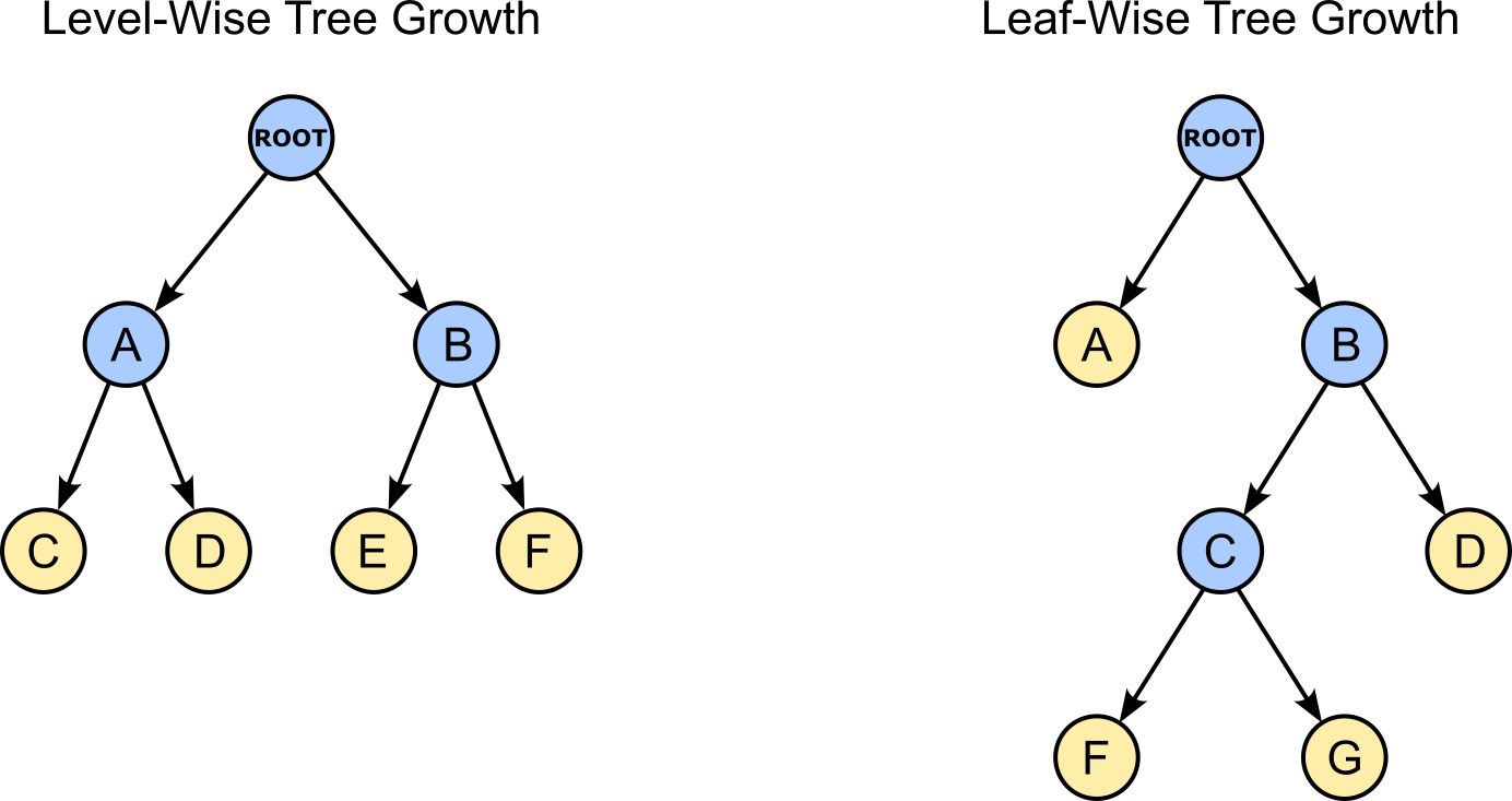
As a result, the tree does not grow uniformly level by level. Instead, it grows where it is most needed. Branches that capture difficult or poorly modeled regions of the data may become much deeper than others, while regions that are already modeled well may remain shallow. This allows the model to focus its complexity on the parts of the feature space where it can achieve the largest reduction in error, often leading to better predictive performance with the same number of leaves compared to level-wise growth.
To determine the next leaf to split, LightGBM finds and keeps track of the best split for each current leaf in the tree — keep in mind that each split is associated with some kind of score (e.g., information gain). The leaf with the highest score is then chosen to be split next to create two new leaf nodes, for which LightGBM again computes their best splits and associated scores. To give an example, consider the small example tree as shown below.
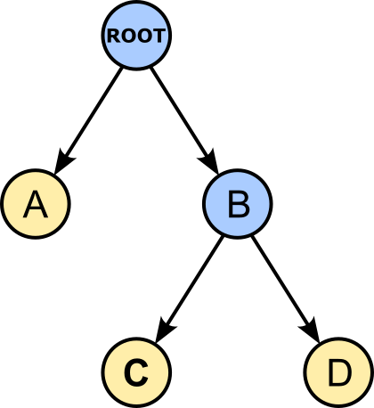
In this tree, Nodes $A$, $C$, and $D$ are the current leaves. This means that LightGBM has computed the best split for all three nodes. Assuming our example dataset with $2$ features, and $3$ bins for each feature, the resulting statistics may look as follows:
| Leaf | Best Split | Score |
|---|---|---|
| A | Feature $x_1$, Bin 2 | 1.5 |
| C | Feature $x_1$, Bin 1 | 9.2 |
| D | Feature $x_2$, Bin 1 | 0.8 |
Since Leaf $C$ has the highest score, it will be the next leaf to be split based on the best split as recorded. This will result in two new leaves, say, $E$ and $F$; as shown in the figure below.
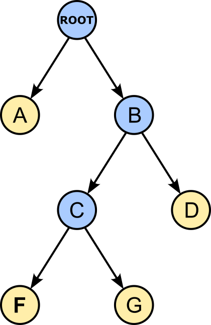
Now that the tree has two new leaves, LightGBM now computes the best splits for $E$ and $F$ to update its leaf statistics. Of course, now that Node $C$ is no longer a leaf, it can in turn be removed from the statistics. Thus, the resulting statistic might now look as shown in the table below.
| Leaf | Best Split | Score |
|---|---|---|
| A | Feature $x_1$, Bin 2 | 1.5 |
| D | Feature $x_2$, Bin 1 | 0.8 |
| E | Feature $x_1$, Bin 2 | 4.2 |
| F | Feature $x_2$, Bin 2 | 2.5 |
The next leaf that LightGBM will split is Leaf $E$ since it has the highest score among all $4$ current leaves. This split will result again in $2$ new leaves, and this process continues until the maximum about leaves — a hyperparameter of LightGBM: num_leaves — is reached. At this point, the training stops.
Both level-wise and leaf-wise tree growth are widely used strategies in gradient boosting and each offers distinct advantages. Level-wise growth tends to produce balanced trees, is less prone to overfitting, and is easier to parallelize, whereas leaf-wise growth allocates model complexity more efficiently by focusing on the regions of the feature space that offer the largest reduction in loss. The table provides some general comparison.
| Aspect | Level-wise Growth | Leaf-wise Growth |
|---|---|---|
| Tree structure | Produces relatively balanced trees. | Produces potentially unbalanced trees with deep branches. |
| Use of model complexity | Distributes splits evenly across the tree. | Concentrates splits where they reduce the loss the most. |
| Training loss | May require more splits to achieve the same reduction in loss. | Often achieves lower training loss with the same number of leaves. |
| Predictive performance | Generally strong and robust. | Often achieves higher accuracy, especially on large datasets. |
| Overfitting risk | Lower, due to balanced growth and implicit regularization. | Higher, as deep branches can fit noise in the training data. |
| Training efficiency | May spend splits on low-gain regions of the feature space. | Allocates splits to the most informative regions first. |
| Parallelization | Easier to parallelize because all nodes at a level are processed together. | More difficult because growth depends on the globally best leaf. |
| Control of complexity | Naturally controlled by tree depth. | Typically controlled using num_leaves, often together with max_depth. |
| Interpretability | More regular and easier to visualize. | Can produce asymmetric trees that are harder to interpret. |
| Main advantage | Robustness, balanced trees, lower risk of overfitting. | More efficient use of splits and often better predictive performance. |
| Main disadvantage | May waste splits on regions that offer little improvement. | More prone to overfitting and can produce very deep branches. |
Consequently, neither strategy is universally superior. The choice between them depends on the characteristics of the dataset, the desired trade-off between predictive performance and robustness, and the computational constraints of the application.
Efficient Data Handling
A primary design goal of LightGBM is to improve computational efficiency and scalability, enabling gradient boosting to be applied effectively to very large datasets. To achieve this, LightGBM not only employs histogram-based split finding and a leaf-wise tree growth strategy, but also introduces two additional optimization techniques: Gradient-based One-Side Sampling (GOSS) and Exclusive Feature Bundling (EFB). These methods further reduce the computational and memory requirements of training by decreasing the number of training instances and features that need to be processed, respectively, while maintaining predictive performance.
Gradient-based One-Side Sampling (GOSS)
Gradient-based One-Side Sampling (GOSS) is based on the observation that, during boosting, samples with large gradients are generally more informative than samples with small gradients. A large gradient indicates that the current model is making a substantial error for that observation, whereas a small gradient suggests that the observation is already predicted reasonably well — the magnitude of a gradient depends on its absolute value but not its sign (i.e., distance from $0$). Instead of building histograms using all training samples that reach a node, GOSS first partitions the samples according to the magnitude of their gradients. Let's illustrate this using our example dataset and sort it with respect to the absolute value of the gradient.
| AGE | INC | Bin/AGE | Bin/INC | LIMIT $y_i$ | $F_{0}(\mathbf{x}_i)$ | $g_{i}^{(1)}$ | $h_{i}^{(1)}$ | |
|---|---|---|---|---|---|---|---|---|
| 3 | 31 | 55,000 | 1 | 1 | 1,400 | 1,000 | -400 | 1 |
| 6 | 41 | 47,000 | 2 | 1 | 600 | 1,000 | 400 | 1 |
| 9 | 58 | 33,000 | 2 | 0 | 600 | 1,000 | 400 | 1 |
| 10 | 27 | 65,000 | 0 | 2 | 1,300 | 1,000 | -300 | 1 |
| 2 | 45 | 92,000 | 2 | 2 | 1,200 | 1,000 | -200 | 1 |
| 4 | 52 | 38,000 | 2 | 1 | 900 | 1,000 | 100 | 1 |
| 7 | 22 | 21,000 | 0 | 0 | 900 | 1,000 | 100 | 1 |
| 8 | 36 | 75,000 | 1 | 2 | 1,100 | 1,000 | -100 | 1 |
| 1 | 24 | 28,000 | 0 | 0 | 1,000 | 1,000 | 0 | 1 |
| 5 | 29 | 120,000 | 1 | 2 | 1,000 | 1,000 | 0 | 1 |
To decide which samples to consider for the training, LightGBM uses two hyperparameters:
top_rate: the fraction of data with large gradients to keep (typical value: $0.2$)other_rate:the fraction of data with small gradients randomly sampled from the remaining pool (typical value $0.1$ — of the remaining 80%)
For our very small example dataset, let's assume top_rate=0.4 and other_rate=0.5. This means that we use the $4$ samples with the largest gradients (Samples 3, 6, 9, 10) and $3$ out of the remaining $6$ samples (e.g., Samples 2, 5, 8) to form the dataset for training a tree.
One important thing to consider is that this sampling means that we need to compensate for the reduced number of low-gradient observations. To ensure that the resulting statistics remain representative of the full dataset, the gradients and Hessians of the sampled low-gradient instances are multiplied by a scaling factor as the reciprocal of other_rate. Thus, with another rate of $0.5$ for our example, we need to scale the low-gradients instances by a factor of $2$. After performing GOSS the two histograms for our examples dataset would look like:
| Bin | Samples | $\sum g_{i}^{(1)}$ | $\sum h_{i}^{(1)}$ |
|---|---|---|---|
| 0 | 10 | $(-300) = -300$ | $(1) = 1$ |
| 1 | 3, 5, 8 | $(-400+2\cdot0-2\cdot 100) = -600$ | $(1 + 2\cdot 1 + 2\cdot 1) = 5$ |
| 2 | 2, 6, 9 | $(2\cdot -200+400+400) = 400$ | $(2\cdot 1 + 1 + 1) = 4$ |
| Bin | Samples | $\sum g_{i}^{(1)}$ | $\sum h_{i}^{(1)}$ |
|---|---|---|---|
| 0 | 9 | $(400) = 400$ | $(1) = 1$ |
| 1 | 3, 6 | $(-400+400) = 0$ | $(1 + 1) = 2$ |
| 2 | 2, 5, 8, 10 | $(-200+0-100-300) = -600$ | $(2\cdot 1 + 2\cdot 1 + 2\cdot 1 + 1) = 7$ |
Notice that the resulting $\sum h_{i}^{(1)}$ values in each histogram still sum to $1$, like in the histograms without GOSS (see above). This shows how the scaling ensures that the statistics with GOSS are still representative of the whole dataset.
In principle, a bin might be empty after GOSS. This can happen if the bin contains only low-gradient samples, and none of them gets randomly sampled to be considered for the training. In this case, both the sum gradients and Hessians are $0$. However, in practice, this is usually not a problem. If a bin has no contributing samples, it contains no information that could help determine a split anyway. The only potential issue is that if GOSS is very aggressive, some bins may become sparsely represented, making the histogram a noisier approximation of the full data. This is one reason why other_rate is typically not chosen to be extremely small.
The sampled dataset is then used in exactly the same way as in the standard histogram-based procedure. The primary benefit of GOSS is that it significantly reduces the number of samples that need to be processed when constructing gradient histograms. By retaining all high-gradient instances, which contain the most information about the model's current errors, and only a weighted subset of low-gradient instances, GOSS preserves the statistics that are most relevant for split selection while substantially reducing computational cost. As a result, histogram construction and tree training become considerably faster, often with only a minor impact on predictive performance — of course, the improvements will be much more substantial compared to our example where we used rather large values for top_rate and other_rate.
Exclusive Feature Bundling (EFB)
EFB addresses the challenge of high-dimensional sparse datasets, which commonly arise after one-hot encoding categorical variables or in text mining applications (e.g., sparse TF-IDF vectors). In such datasets, many features are mutually exclusive, meaning that they are rarely or never non-zero at the same time. EFB exploits this property by combining several mutually exclusive features into a single bundled feature without losing information. As a result, the effective number of features is significantly reduced, leading to lower memory consumption and faster histogram construction and split search. Because the bundled features do not overlap in their non-zero values, the original features can still be distinguished during training.
To illustrate this, recall that our original example dataset contains the feature MARITAL_STATUS (simplified MS); and let's assume it has only the three values "Single", "Married", "Divorced", and "Widowed".
| AGE | INC | MS | LIMIT $y_i$ | |
|---|---|---|---|---|
| 1 | 24 | 28,000 | Single | 1,000 |
| 2 | 45 | 92,000 | Married | 1,200 |
| 3 | 31 | 55,000 | Single | 1,400 |
| 4 | 52 | 38,000 | Divorced | 900 |
| 5 | 29 | 120,000 | Married | 1,000 |
| 6 | 41 | 47,000 | Widowed | 600 |
| 7 | 22 | 21,000 | Single | 900 |
| 8 | 36 | 75,000 | Married | 1,100 |
| 9 | 58 | 33,000 | Divorced | 600 |
| 10 | 27 | 65,000 | Single | 1,300 |
A common way to convert categorical features into numerical ones is via one-hot encoding, which One-hot a categorical feature with $k$ distinct categories into $k$ separate binary features. Each binary feature corresponds to one category and takes the value $1$ if the observation belongs to that category and $0$ otherwise. For our example, one-hot encoding would yield the following transformed dataset — with the $4$ new features MS$_s$ for "Single", MS$_m$ for "Married", MS$_d$ for "Divorced", and MS$_w$ for "Widowed":
| AGE | INC | $\mathbf{MS}_s$ | $\mathbf{MS}_m$ | $\mathbf{MS}_d$ | $\mathbf{MS}_w$ | LIMIT $y_i$ | |
|---|---|---|---|---|---|---|---|
| 1 | 24 | 28,000 | 1 | 0 | 0 | 0 | 1,000 |
| 2 | 45 | 92,000 | 0 | 1 | 0 | 0 | 1,200 |
| 3 | 31 | 55,000 | 1 | 0 | 0 | 0 | 1,400 |
| 4 | 52 | 38,000 | 0 | 0 | 1 | 0 | 900 |
| 5 | 29 | 120,000 | 0 | 1 | 0 | 0 | 1,000 |
| 6 | 41 | 47,000 | 0 | 0 | 0 | 1 | 600 |
| 7 | 22 | 21,000 | 1 | 0 | 0 | 0 | 900 |
| 8 | 36 | 75,000 | 0 | 1 | 0 | 0 | 1,100 |
| 9 | 58 | 33,000 | 0 | 0 | 1 | 0 | 600 |
| 10 | 27 | 65,000 | 1 | 0 | 0 | 0 | 1,300 |
Important: Note that the assumption here is that we get a dataset that already contains one-hot encoded features. Unlike many machine learning algorithms, LightGBM can handle categorical features natively and therefore does not require one-hot encoding as a preprocessing step. Instead, categorical variables can be provided directly to the model, which uses gradient and Hessian statistics to identify effective partitions of the categories during split selection. This often leads to lower memory consumption, faster training, and improved predictive performance, particularly for features with many distinct categories. If you do not one-hot encode the categorical feature and instead tell LightGBM that it is categorical, then LightGBM uses its native categorical feature handling. In that case, EFB is not relevant because there are no separate one-hot encoded features to bundle.
However, assuming we get a dataset with sparse features, the advantage of EFB is that you do not need to manually specify which features are mutually exclusive. Instead, LightGBM automatically analyzes the sparsity patterns in the training data and identifies features that rarely or never take nonzero values simultaneously. Based on this analysis, it groups compatible features into bundles, thereby reducing the effective dimensionality of the dataset while preserving the information required for model training. For example, based on one-hot encoding, LightGBM will create the following bundle feature:
| AGE | INC | BUNDLE | $y_i$ | |
|---|---|---|---|---|
| 1 | 24 | 28,000 | 1 | 1,000 |
| 2 | 45 | 92,000 | 2 | 1,200 |
| 3 | 31 | 55,000 | 1 | 1,400 |
| 4 | 52 | 38,000 | 3 | 900 |
| 5 | 29 | 120,000 | 2 | 1,000 |
| 6 | 41 | 47,000 | 4 | 600 |
| 7 | 22 | 21,000 | 1 | 900 |
| 8 | 36 | 75,000 | 2 | 1,100 |
| 9 | 58 | 33,000 | 3 | 600 |
| 10 | 27 | 65,000 | 1 | 1,300 |
where:
- 1 = Single
- 2 = Married
- 3 = Divorced
- 4 = Windowed
A consequence of this bundling is that the resulting feature introduces an ordering of the categories, suggesting relationships such as Single < Married < Divorced < Widowed, even though no such natural ordering exists. This means that during training a tree, only the following binary partitions are possible:
- BUNDLE $ < 1.5\ \Rightarrow$ {Single} vs. {Married, Divorced, Widowed}
- BUNDLE $ < 2.5\ \Rightarrow$ {Single, Married} vs. {Divorced, Widowed}
- BUNDLE $ < 3.5\ \Rightarrow$ {Single, Married, Divorced} vs. {Widowed}
In contrast, not possible would be, for example, the split {Single, Widowed} vs. {Married, Divorced}. Although this is a principle limitation, LightGBM prioritizes efficiency to be able to deal with very large datasets. Additionally, Decision Trees are generally more robust to this issue than many other machine learning models. Since trees recursively partition the feature space, they can use multiple splits to isolate individual category values or groups of values. Consequently, even if the imposed ordering is not meaningful, a sufficiently deep tree can often approximate the desired partitions, reducing the negative impact of the encoding. However, this may require more splits than methods that natively support categorical features.
Important: Just to emphasize it again, LightGBM handles categorical features natively using a highly optimized, gradient-based algorithm — which is beyond the scope here. This, for our example dataset, if "Single", "Married", "Divorced", and "Widowed" originate from a single categorical variable, it is generally preferable to provide that variable directly as a categorical feature. EFB becomes relevant when we start off with very sparse features such as features generated by one-hot encoding.
Summary (GMBs vs LightGBM): Compared to traditional GBMs, LightGBM introduces several innovations aimed primarily at improving computational efficiency and scalability. Most notably, it employs histogram-based split finding, which reduces the number of candidate split points by discretizing numerical features into bins, and a leaf-wise tree growth strategy that focuses model complexity on the regions of the feature space with the largest potential reduction in loss. In addition, LightGBM introduces Gradient-based One-Side Sampling (GOSS) to reduce the number of training instances used during histogram construction and Exclusive Feature Bundling (EFB) to reduce the effective dimensionality of sparse datasets. Together, these techniques enable LightGBM to train significantly faster and use less memory than traditional GBMs while maintaining competitive predictive performance on large-scale datasets. That table below provides a direct comparison of the core aspects of GBMs and LightGBM.
| Aspect | Traditional GBM | LightGBM |
|---|---|---|
| Primary objective | Accurate gradient boosting using sequentially trained decision trees. | Improve the efficiency and scalability of gradient boosting for large datasets. |
| Split finding | Evaluates splits using raw feature values and many candidate thresholds. | Uses histogram-based split finding on discretized feature bins. |
| Feature representation | Operates directly on original feature values. | Quantizes numerical features into a fixed number of bins before training. |
| Tree growth strategy | Typically grows trees level-wise (depth-wise). | Grows trees leaf-wise by always splitting the leaf with the highest gain. |
| Candidate split points | Potentially thousands or millions per feature. | At most $b-1$ split points per feature, where $b$ is the number of bins. |
| Training samples used | All samples are typically used when evaluating splits. | Can optionally use Gradient-based One-Side Sampling (GOSS) to focus on informative samples. |
| Feature dimensionality | Uses all features as provided. | Can reduce dimensionality through Exclusive Feature Bundling (EFB). |
These characteristics of LightGBM greatly reduce the memory consumption and speed up the training of LightGBM models (compared to traditional GBMs), making them much more scalable when handling large datesets with high-dimensional feature spaces. However, the risk of overfitting is potentially higher due to aggressive leaf-wise growth, requiring appropriate regularization. Furthermore, histogram-based splitting and Exclusive Feature Bundling (EFB) can negatively affect the precision. LightGBM therefore shines when working with very large and sparse datasets where efficiency is a primary concern. For small to medium-sized datasets where training speed is less critical, traditional GBMs (or XGBoost) might remain the preferred choice.
CatBoost
CatBoost is a gradient boosting algorithm specifically designed to handle categorical features effectively and efficiently without requiring extensive preprocessing such as one-hot encoding. While it retains the core boosting framework of traditional Gradient Boosted Machines (GBMs), CatBoost introduces several key innovations that address important sources of bias and inefficiency in standard implementations.
First, ordered target encoding (also known as ordered target statistics) transforms categorical features into numerical representations while avoiding target leakage. Second, ordered boosting mitigates the prediction shift that arises in conventional boosting by computing gradients using predictions that do not depend on the target of the current training example. Finally, CatBoost employs oblivious trees, a symmetric tree architecture that improves computational efficiency, facilitates the implementation of ordered boosting, and provides additional regularization. Together, these innovations enable CatBoost to achieve strong predictive performance, particularly on datasets containing high-cardinality categorical variables.
Ordered Target Encoding
An alternative to one-hot encoding for converting categorical variables into numerical features is target encoding. Rather than creating a separate binary feature for each category, target encoding replaces each category with a statistic derived from the target variable, such as the mean target value of all samples belonging to that category. For example, in a regression problem, each category may be represented by the average target value observed for that category, while in binary classification it may be represented by the proportion of positive instances. As a result, target encoding preserves the information contained in categorical variables without increasing the dimensionality of the dataset, making it particularly attractive for features with many distinct categories.
Mathematically, the target-encoded value of some categorical feature $k$ for data sample $\mathbf{x}_i^{(k)}$ is defined as:
where $\mathbb{I}(\mathbf{x}_j^{(k)} = \mathbf{x}_i)^{(k)}$ is $1$ if both samples $\mathbf{x}_i$ and $\mathbf{x}_j$ have the same value for the $k$-th feature. This means that the denominator is simply the number of data samples in the same category, i.e., the data samples that share the same value for the $k$-th feature. The table below shows the result after target encoding MARITAL_STATUS (MS).
| AGE | INC | $\mathbf{MS}_{target}$ | LIMIT $y_i$ | |
|---|---|---|---|---|
| 1 | 24 | 28,000 | 1,150 | 1,100 |
| 2 | 45 | 92,000 | 1,100 | 1,200 |
| 3 | 31 | 55,000 | 1,150 | 1,400 |
| 4 | 52 | 38,000 | 750 | 900 |
| 5 | 29 | 120,000 | 1,100 | 1,000 |
| 6 | 41 | 47,000 | 600 | 600 |
| 7 | 22 | 21,000 | 1,150 | 900 |
| 8 | 36 | 75,000 | 1,100 | 1,100 |
| 9 | 58 | 33,000 | 750 | 600 |
| 10 | 27 | 65,000 | 1,150 | 1,300 |
For example, there are $3$ samples with the value "Married" for MARITAL_STATUS (MS). This means that the encoded value is computed as $(1,200+1,000+1,100)/3 = 1,100$. Apart from just converting the feature values for the training data, we also need to remember the mapping — here: {"Single: 1,150, "Married": 1,100, "Divorced": 750, , "Widowed": 6000} — to encode the marital status for unseen samples during inference.
A fundamental limitation of basic target encoding is that the encoded feature value for a sample $x_i$ is computed using category-level statistics that include the sample's own target value $y_i$. As a result, the transformed feature is no longer independent of the target variable. In other words, information from $y_i$ is implicitly fed back into the feature representation of $x_i$, creating a form of target leakage. Since the model is trained on features that already contain information about the outcome it is trying to predict, performance estimates can become overly optimistic.
This issue is particularly pronounced for categories with only a small number of observations. When a category contains very few samples, the category mean is strongly influenced by each individual target value. In the extreme case of a category appearing only once, the encoded value is determined entirely by that sample's target. Consequently, the encoded feature reveals substantial information about $y_i$, effectively leaking part of the label into the input features. This leakage can lead to overfitting and poor generalization. To address, some basic extensions to basic target encoding are commonly employed in practice:
Smoothing: Smoothing reduces the variance and leakage of target encoding by combining the category-specific target mean with the global target mean. Categories with many observations receive an encoded value close to their own mean, while categories with few observations are shrunk toward the overall mean. This prevents small categories from producing extreme or overly target-dependent encoded values and improves generalization.
Leave-one-out (LOO) target encoding: LOO target encoding reduces target leakage by computing the encoded value for each sample using the category mean after excluding that sample's own target value. As a result, the encoded feature no longer directly depends on $y_i$, which decreases the amount of information leaked from the target into the input feature while still capturing category-level target information.
Cross-validated target encoding: Cross-validated target encoding splits the training data into, say, 10 folds or blocks. The encoded feature values for sample $\mathbf{x}_i$ is computed using only the mean across all 9 folds sample $\mathbf{x}_i$ is not in. This also ensures that a sample's encoded value is derived from data that does not include its own target value, with even less correlation than LOO target encoding, resulting in a more realistic and robust feature representation.
Although smoothing, leave-one-out encoding, and cross-validated target encoding substantially reduce target leakage, they do not eliminate it completely. Residual dependencies between the encoded feature values and the target can still remain, especially in small or infrequent categories. While these effects may appear negligible in isolation, they can become amplified in boosting algorithms, which sequentially train a large number of dependent trees. Since each tree is fitted to the errors of the previous ones, even small amounts of leaked target information can accumulate throughout the boosting process, which again increases the risk of overfitting and overly optimistic performance estimates.
Because even small amounts of target leakage can accumulate in boosting algorithms, CatBoost introduces ordered target encoding to more closely mimic the conditions encountered during inference. At prediction time, the target value of a new sample is unknown, so any encoding procedure that directly or indirectly uses that target creates a mismatch between training and inference. CatBoost addresses this issue by constructing encoded features in a way that prevents a training sample from using information derived from its own target or from the targets of samples that conceptually come "after" it.
The basic idea is to impose a random ordering on the training data and compute the encoded value for each sample using only the target values of earlier samples in that ordering. Consequently, when encoding a sample, only information that would have been available at that point is used, making the process resemble the prediction of a previously unseen observation. This substantially reduces target leakage and produces more reliable categorical feature representations, particularly when combined with boosting methods that are highly sensitive to even minor leakage effects.
The formula below shows the main extension to basic target encoding — notice how the upper bound of the sums is now $i-1$ (instead of $N$ as before), meaning that we consider only the data sample combining before $\mathbf{x}_i$ (instead of all data samples).
Side note: The full formula is a bit more complex since CatBoost also performs smoothing, but here we want to focus on the key innovation only.
In some sense, this imposed ordering is entirely artificial: there is usually no natural sequence in the training data. Consequently, the encoded value assigned to a sample depends on its position within the chosen permutation. This effect is particularly pronounced for samples appearing early in the order, as only a small number of preceding observations are available to estimate category statistics. As a result, a single ordering can introduce additional variance into the encoded features.
To reduce this sensitivity, CatBoost uses multiple random permutations of the training data during learning. In practice, only a relatively small number of $K$ permutations is typically required (often on the order of a few to several permutations, say $K = 4\dots10$, depending on the dataset size and training configuration). Therefore, CatBoost calculates $K$ distinct encodings for that single categorical column. However, when training a tree, CatBoost randomly picks only one of the $K$ permutations. The table below shows an example of using ordered target encoding with $K=4$ on our example dataset. Note that these results involve some smoothing, but the main take-away message is to show how the encoded values for each sample change across permutations.
| AGE | INC | $\mathbf{MS}_{target}^{(1)}$ | $\mathbf{MS}_{target}^{(2)}$ | $\mathbf{MS}_{target}^{(3)}$ | $\mathbf{MS}_{target}^{(4)}$ | LIMIT $y_i$ | |
|---|---|---|---|---|---|---|---|
| 1 | 24 | 28,000 | 800.00 | 1,000.00 | 950.00 | 1,000.00 | 1,100 |
| 2 | 45 | 92,000 | 1,100.00 | 1,150.00 | 1,000.00 | 1,175.00 | 1,200 |
| 3 | 31 | 55,000 | 1,000.00 | 1,175.00 | 1,100.00 | 1,000.00 | 1,400 |
| 4 | 52 | 38,000 | 1,000.00 | 1,100.00 | 1,000.00 | 1,000.00 | 900 |
| 5 | 29 | 120,000 | 1,000.00 | 1,000.00 | 1,000.00 | 950.00 | 1,000 |
| 6 | 41 | 47,000 | 1,000.00 | 1,100.00 | 950.00 | 1,000.00 | 600 |
| 7 | 22 | 21,000 | 1,133.33 | 950.00 | 1,150.00 | 1,100.00 | 900 |
| 8 | 36 | 75,000 | 1,000.00 | 1,000.00 | 1,066.67 | 1,000.00 | 1,100 |
| 9 | 58 | 33,000 | 1,050.00 | 1,100.00 | 1,000.00 | 1,066.67 | 600 |
| 10 | 27 | 65,000 | 1,175.00 | 1,000.00 | 1,050.00 | 1,100.00 | 1,300 |
Take a look at the results or Sample 6 which is the only sample with the value "Widowed" for the marital status. As such, no category mean can be computed and the encoded value depends completely on the mean of all previous samples due to smoothing.
Important: The permutations are only a training-time mechanism used to obtain unbiased target statistics and reduce target leakage. At inference time, CatBoost does not use permutations of the test data. After training, CatBoost has learned "global" target statistics for the categorical features across all samples in the training data. To encode a new sample, the model computes these statistics using all available training data, since the training targets are known and there is no risk of leaking information from the test sample itself. In short, during inference, CatBoost behaves identically to standard target encoding (apart from that CatBoost uses smoothing by default).
Ordered Boosting
Ordered target encoding addresses the data leakage when converting categorical data into numerical based on the fundamental idea behind target encoding. However, even if the original dataset contained only numerical data to begin with, the basic concept of boosting causes some form of data leakage. The leakage in traditional boosting does not happen because of an explicit mistake like accidentally leaving the target variable in your training features. Instead, it is a structural leakage built into the optimization loop itself, often referred to as prediction shift.
Recall that in gradient boosting, trees are trained sequentially, where each new tree is built to predict the gradients (residuals) of the loss function calculated from the current learners' predictions. More specifically, we perform the following core steps in any given iteration
Predict: Use the current ensemble of trees to predict $F_{m}(\mathbf{x}_i)$ for every sample $\mathbf{x}_i$ in the training set; recall: $\ F_{m}(\mathbf{x}_i) = F_{m-1}(\mathbf{x}_i) + \eta f_t(\mathbf{x}_i)$
Calculate gradients: Compute the gradient $g_i$ (or pseudo-residual $r_i$) for each sample $\mathbf{x}_i$ using its true target $y_i$ and the prediction $\hat{y}_i$; recall: $\ g_{i}^{(m)} = r_{i}^{(m)} = y_i - F_{m}(\mathbf{x}_i)$
Train new tree: Build a new tree $\ f_t\ $ to fit these gradients for all training samples.
The leakage happens because the exact same dataset is reused in every single step of this loop. The issue is that $F_{t-1}$ was trained on all training examples, including example $\mathbf{x}_i$. This means that $F_{t-1}(\mathbf{x}_i)$ already depends on $y_i$, and thus the residual $r_i^{(m)}$ depends on $y_i$ twice:
- Directly through the $y_i$ term
- Indirectly because $F_{t-1}$ was learned using $y_i$
In short, during training, $F(x_i)$ depends on $y_i$ for all training samples $\mathbf{x}_i$. However, during inference, assuming an unseen data sample $\mathbf{x}$, $F(\mathbf{x})$ cannot depend on the unknown target $y$, which is what we want to predict. Therefore the gradients are computed under a different distribution than the one the model will face after deployment resulting in the so-called prediction shift. In many algorithms, using the same data to fit parameters and compute residuals is standard, including Linear Regression, Random Forests, XGBoost, LightGBM, etc. The resulting bias is often small and acceptable. CatBoost's authors showed that for boosting, especially with many iterations and categorical features, the bias accumulates and can hurt generalization. So CatBoost explicitly tries to eliminate it.
Ordered boosting applies the same "time-series" philosophy of ordered target encoding to the actual gradient calculation and tree structural learning. Instead of training a single set of trees on the entire dataset, ordered boosting trains and maintains multiple parallel models based on virtual permutations of the data. The core idea is as follows:
Random permutations: CatBoost generates several independent random permutations of the training data. This establishes an artificial "historical order" for the rows.
Parallel sub-models: For a given permutation, CatBoost maintains a sequence of submodels $M_1$, $M_2$, $M_3$, ..., $M_n$; where model $M_i$ is trained only using the first $i$ samples in that permutation.
Leakage-free gradients: When the algorithm needs to calculate the gradient (residual) for sample $\mathbf{x}_{i+1}$ to train the next tree, it does not look at the current global ensemble, but calculates the residual of sample $\mathbf{x}_{i+1}$ using model $M_i$.
Because Model $M_i$ was trained strictly on samples $\mathbf{x}_1$ to $\mathbf{x}_i$, it has absolutely no knowledge of $y_{i+1}$. The gradient for sample $\mathbf{x__{i+1}$ is completely unshifted and behaves exactly as if it were an independent test data point.
Of course, a naive implementation of ordered boosting would require maintaining a separate model for every training example, where the prediction for the $i$-th example is generated by an ensemble trained only on the examples that precede it in a random permutation. For a dataset with $n$ samples, this implies maintaining $n$ different versions of the boosting model and updating them at every iteration, leading to computational and memory costs that grow on the order of $O(n^2)$. Even for moderately sized datasets containing hundreds of thousands or millions of observations, training and storing such a large collection of ensembles would be completely impractical. This is why CatBoost does not implement ordered boosting literally; instead, it introduces a series of approximation techniques (including shared tree structures, multiple permutations, and efficient prefix-based statistics) that closely approximate the ideal ordered procedure while keeping training time and memory usage comparable to conventional gradient boosting methods. However, a deeper discussion would go way beyond the scope of this introductory notebook.
Oblivious (Symmetric) Trees
In a traditional Decision Tree (like those used in XGBoost or LightGBM), each internal node splits independently based on whatever feature maximizes information gain for that specific subset of data. This results in an asymmetric, irregular structure. An asymmetric structure generally refers to a tree with an uneven depth. For example, one path might require evaluating 5 different features to reach a leaf, while another path might reach a final leaf after just 1 split. "Irregularity" refers to the fact that the conditions checked at the same depth level of the tree are completely unrelated. They depend entirely on which branch a data point took.
In contrast, Oblivious Trees (also called Symmetric Trees) are Decision Trees in which all nodes at the same depth use the same splitting rule. In a depth-$d$ Oblivious Tree, the model selects exactly $d$ splits, and every sample is evaluated against those same splits in the same order. As a result, the tree forms a perfectly balanced structure with $2^d$ leaves, where each leaf corresponds to a unique combination of split outcomes. The figure below compares a standard Decision Tree and a Oblivious Tree but showing them only until a depth of $2$ (this includes that leaves are omitted!); here, if two inner nodes have the same color, they are using the exact same decision (i.e., same feature and same threshold).
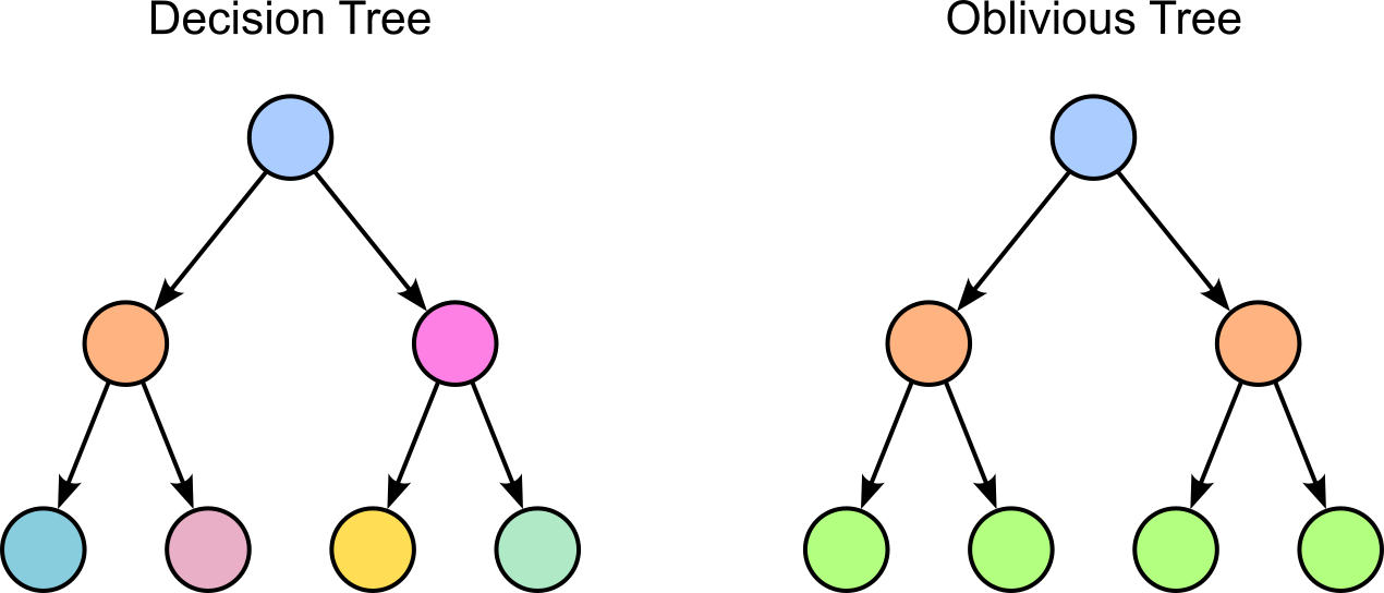
CatBoost uses Oblivious Trees for both computational efficiency and regularization. Their highly structured form allows tree traversal and leaf assignment to be implemented very efficiently, which is particularly important because CatBoost's ordered boosting algorithm requires maintaining and updating multiple prefix-based prediction statistics during training. The symmetric structure also makes it easier to share tree topologies across these computations and enables highly optimized CPU and GPU implementations. From a statistical perspective, oblivious trees are more constrained than conventional CART trees, reducing the model's flexibility and helping to prevent overfitting. Consequently, they typically exhibit a favorable bias-variance tradeoff, contributing to CatBoost's strong generalization performance while keeping training computationally tractable.
Quick comparison
The effectiveness of gradient boosting has led to the development of several advanced algorithms that extend the basic Gradient Boosting Machine (GBM) framework to address specific challenges and improve performance. While all of these methods retain the core idea of sequentially adding weak learners to correct the errors of an existing ensemble, they introduce novel techniques to enhance accuracy, efficiency, scalability, or robustness. For example, XGBoost incorporates second-order optimization, regularization, and highly optimized parallelized training procedures to improve predictive performance and computational efficiency. LightGBM focuses on scalability for large datasets through innovations such as histogram-based splitting, leaf-wise tree growth, and efficient feature bundling. CatBoost, in turn, is specifically designed to handle categorical features effectively through ordered target encoding, ordered boosting, and oblivious trees. The table below provides a high-level comparison.
| Feature | GBM | XGBoost | LightGBM | CatBoost |
|---|---|---|---|---|
| Gradient boosting | ✓ | ✓ | ✓ | ✓ |
| Regularization | Basic | Strong | Strong | Strong |
| Uses Hessians | Usually no | Yes | Yes | Yes |
| Training speed | Slow | Fast | Very fast | Fast |
| Memory efficiency | Low | Medium | High | Medium |
| Large datasets | Fair | Good | Excellent | Good |
| Categorical features | Manual encoding | Manual encoding | Limited support | Excellent |
| Default performance | Moderate | Strong | Strong | Strong |
| Risk of overfitting | Moderate | Moderate | Higher (leaf-wise growth) | Lower |
Although there is typically no reliable way to say a-priori which model will perform best on a specific dataset for a specific task, here are some very crude rules of thumb to gauge which model is more suitable in which situation.
- Learning gradient boosting concepts: GBM
- General-purpose tabular data: XGBoost
- Very large datasets or speed-critical training: LightGBM
- Many categorical features: CatBoost
In practice, of course, you will likely try and compare various models. Despite their strong predictive performance, however, gradient boosting methods are generally more computationally expensive than many other machine learning models. Unlike models that can be trained in a single optimization step or whose components can be learned independently, boosting algorithms build learners sequentially, with each iteration depending on the results of all previous iterations. As a result, training often requires constructing hundreds or even thousands of trees, leading to substantial computational and memory demands, particularly for large datasets.
Summary
This notebook introduced the fundamental ideas behind boosting, a powerful ensemble learning strategy that combines many weak learners into a strong predictive model. Unlike bagging methods, which train models independently and aggregate their predictions, boosting constructs models sequentially, with each new learner focusing on the mistakes made by the existing ensemble. We examined two of the most influential boosting paradigms: AdaBoost, which adapts by reweighting training examples so that misclassified observations receive greater attention in subsequent iterations, and Gradient Boosting Machines (GBMs), which iteratively fit new learners to the residual errors or gradients of the current model.
Building on these foundations, we explored how modern gradient boosting algorithms extend the original GBM framework. While traditional GBMs already achieve excellent predictive performance, practical challenges such as computational efficiency, scalability, overfitting, and the handling of categorical features have motivated the development of more sophisticated methods. Algorithms such as XGBoost, LightGBM, and CatBoost retain the core principle of sequential error correction while introducing innovations that make boosting faster, more robust, and better suited to different types of data and machine learning tasks.
Boosting models are among the most successful machine learning techniques for structured (tabular) data, where they frequently achieve state-of-the-art results in both classification and regression problems. Their ability to model complex nonlinear relationships, capture feature interactions automatically, and adaptively focus on difficult observations often allows them to outperform simpler linear models as well as many alternative machine learning approaches. As a result, boosting algorithms have become a standard tool in applied machine learning, data science competitions, and industrial predictive modeling applications.
Despite their impressive performance, boosting methods also come with important trade-offs. Compared with many other model families, they are computationally more expensive, require careful hyperparameter tuning, and can be more difficult to interpret. Understanding the strengths and limitations of boosting, as well as the key innovations underlying popular frameworks such as XGBoost, LightGBM, and CatBoost, is therefore an essential skill for practitioners seeking to build high-performing predictive models on real-world datasets.