Disclaimer: This Jupyter Notebook contains content generated with the assistance of AI. While every effort has been made to review and validate the outputs, users should independently verify critical information before relying on it. The SELENE notebook repository is constantly evolving. We recommend downloading or pulling the latest version of this notebook from Github.
Data Normalization — Motivation & Overview
Data normalization is one of the most fundamental but also often underestimated steps in data analysis and machine learning. In theory, many algorithms are presented as clean mathematical procedures operating on well-behaved numerical inputs. In practice, however, real-world datasets rarely arrive in such a convenient form. Features may differ drastically in scale, units, or distribution; some variables may range between $0$ and $1$, while others span thousands or millions. Before building models or drawing conclusions, it is therefore essential to understand what "unnormalized" data means and why it is the norm rather than the exception in applied settings.
Unnormalized data appears in many forms. Features can have vastly different magnitudes (e.g., income in dollars versus age in years), incomparable units (e.g., temperature, distance, and counts in the same dataset), or highly skewed distributions with extreme outliers. Even when numerical ranges look similar, differences in variance or distribution shape can still distort downstream computations. In real-world domains such as finance, healthcare, engineering, and social sciences, heterogeneous data sources and measurement scales make unnormalized features a common and recurring challenge.
The consequences of ignoring normalization can be severe. Many machine learning and data analysis methods rely explicitly or implicitly on distances, dot products, gradients, or variance-based criteria. Algorithms such as k-nearest neighbors, k-means clustering, principal component analysis, and gradient-based neural networks can become dominated by features with larger scales. This can lead to unstable training dynamics, slower convergence, biased parameter estimates, and misleading interpretations. In short, the model may learn patterns that reflect measurement scale rather than meaningful structure in the data.
To address these issues, a range of normalization strategies has been developed. Common approaches include min-max scaling, standardization (z-score normalization), robust scaling based on medians and interquartile ranges, and logarithmic or power transformations for skewed features. Each method serves different purposes and makes different assumptions about the data distribution. Choosing an appropriate strategy requires understanding both the dataset and the learning algorithm being used.
Mastering normalization is therefore not merely a technical preprocessing step but a prerequisite for obtaining reliable, interpretable, and reproducible results. A solid understanding of why normalization matters, when it is needed, and how to apply it correctly ensures that models capture genuine structure in the data rather than artifacts of scale. In practice, careful normalization often makes the difference between unstable experimentation and robust, trustworthy analysis.
Setting up the Notebook
This notebook does not contain any code, so there is no need to import any libraries or other external code.
What is "Unnormalized" Data
In machine learning, unnormalized data generally refers to input features whose numerical scales, ranges, or distributions have not been adjusted to be comparable or well-behaved for learning algorithms. This often means that different features have vastly different magnitudes (e.g., income in thousands versus age in tens), are not centered around zero, or exhibit strong skewness or outliers. As a result, the raw numerical values reflect arbitrary units or measurement choices rather than meaningful relative importance between features. Before looking into the negative effects that unnormalized data may cause, let's first see some examples of unnormalized data why this is a common phenomenon when working with raw data.
Features with Different Scales
Structured, or tabular, data often consists of multiple features that capture different aspects of the same objects or events. These features can have values that vary wildly in scale. To give an example, the table below shows an extract of a healthcare dataset with various measurements as features.
| Patient_ID | Age (years) | Systolic_BP (mmHg) | Cholesterol (mg/dL) | WBC_Count (cells/μL) | Platelet_Count (cells/μL) | Bilirubin (mg/dL) |
|---|---|---|---|---|---|---|
| P001 | 69 | 133 | 238 | 6888 | 218148 | 0.6 |
| P002 | 32 | 153 | 198 | 10310 | 402801 | 0.4 |
| P003 | 89 | 139 | 208 | 9393 | 274243 | 1.2 |
| P004 | 78 | 147 | 164 | 6435 | 401995 | 0.7 |
| P005 | 38 | 111 | 200 | 4600 | 304555 | 0.4 |
| P006 | 41 | 130 | 257 | 6363 | 198555 | 0.9 |
| P007 | 20 | 142 | 204 | 6061 | 406508 | 0.1 |
| P008 | 39 | 121 | 213 | 4241 | 429303 | 1.3 |
| P009 | 70 | 131 | 200 | 6041 | 256530 | 0.7 |
| P010 | 19 | 153 | 170 | 6824 | 230077 | 0.7 |
Without any more elaborate explanation of the different features, the key observation is that the values differ by several orders of magnitude across all features. This is not an isolated example but in fact a very common occurrence in real-world dataset across all kinds of domains. Beyond healthcare and biomedical data, other domains showing this characteristic include:
Finance & economics: In finance and economics, datasets often contain features with extremely different scales. For instance, asset prices can range from just a few units up to around a thousand, while trading volumes commonly span from thousands to hundreds of millions. Market capitalization values can be even larger, reaching into the trillions, whereas interest rates or returns are often tiny fractions, sometimes on the order of 0.01% to 10%. This means that it is not unusual to see tables that mix cents, percentages, and billions all in the same dataset.
Sensor and IoT data: Data stemming from physical devices contain measurements reflecting the diversity of physical phenomena being monitored. For example, temperature readings are typically in the tens of degrees Celsius, while pressure sensors can report values on the order of hundreds of thousands of pascals. Acceleration measurements are usually single-digit meters per second squared, whereas voltages can range from millivolts up to tens of volts. Signal power, whether expressed in decibels or raw counts, can span an even more extreme range, from millionths to millions.
User behavior & web analytics: Web analytics datasets often combine counts, ratios, and timestamps in the same table. For example, page views for a website can range from zero to millions, while click-through rates are fractions between zero and one. Session durations, measured in seconds, typically span from a few seconds up to tens of thousands, and user identifiers or raw timestamps can be extremely large numbers, often exceeding a billion. The presence of raw timestamps is particularly challenging, as their large magnitude can easily dominate calculations if not properly handled.
Demographic & census data: Socio-economic variables often span vastly different scales. For instance, age typically ranges from a few years to over a hundred, while household sizes are usually between one and ten members. Income values can vary from thousands to millions, and net worth can reach into the hundreds of millions, reflecting extreme wealth disparities. Population density is another feature with a wide range, from sparsely inhabited areas with just a few individuals per square kilometer to densely populated urban centers exceeding hundreds of thousands.
Scientific & engineering data: Scientific and engineering datasets often contain features such length measurements can range from nanometers ($10^{9}$ m) to meters, while energy values may be expressed in electronvolts or joules, spanning vastly different magnitudes. Frequencies in these datasets can also vary enormously, from a few hertz to trillions of hertz ($10^8-10^{12}$ Hz), and simulation parameters often represent different physical quantities, each with its own natural scale.
In general, the problem with different scales or magnitudes is that features with very (large) value might dominate a machine learning algorithm; and we will see concrete examples later. In most cases, however, we typically assume that all features are (or at least might be) equally important.
Even if input data are carefully normalized, they can become effectively unnormalized after one or more neural network layers because each layer applies a learned affine transformation followed by a non-linear activation. The linear part (weights and biases) can rescale and shift activations in arbitrary ways during training, so the distribution of activations may drift in mean and variance as they propagate through the network. As parameters are updated, this drift can change over time, meaning that later layers see inputs whose scale and distribution are neither fixed nor well controlled.
Non-linear activation functions further exacerbate this effect by reshaping the activation distribution in a non-uniform way, for example by clipping negative values (ReLU) or compressing values into a bounded range (sigmoid, tanh). Across multiple layers, these transformations compound, potentially leading to exploding or vanishing activations and unstable gradients. This is why techniques such as Batch Normalization or layer normalization are often introduced: they re-normalize intermediate activations to maintain stable distributions and make training deeper networks more reliable.
Features with Different Units
Basically all domains we have mentioned above — healthcare & biomedical, finance & economics, sensor and IoT data, user behavior & web analytics, demographic & census data, scientific & engineering data — contain features with different units, either base units (e.g., mass, length, time, temperature, charge) or derived units (e.g., speed, acceleration, work, energy, pressure). We already saw that different units often have very different orders of magnitudes which can cause problems when building machine learning models.
That being said, just because two features have values of similar scale or magnitude does not automatically mean that both features can be considered being normalized. To illustrate the problem, consider a healthcare dataset for training a model to predict the risk of a certain disease based on patients' biomedical data including the resting heart rate in beats per minute (BPM) and the body temperature in degrees Celsius (°C). For a normal adult the resting heart rate is typically in the range of 60 to 100 BPM, and the body temperature is typically in the range of 36 to 37 °C (depending on how it is measured). This both the heart rate and the body temperature are generally in the same order of magnitude.
The issue now is that these two measurements have different sensitivities. While a difference in the resting heart rate of 2-3 BPM can be considered negligible, a difference of 2-3 °C in body temperature can mean the difference between life and death. In other words, the change of BPM and °C by 1 unit is semantically not comparable. However, most machine learning algorithms treat numbers as pure numbers and have no notion of physical meaning or units and therefore assume that changing different features by the same amount is comparable. In short, "unnormalized" does not just mean "numbers are large or small". It also means features are not on a comparable scale in terms of meaning, variance, and influence on the model, which often happens precisely when features come from different domains and units, even if their raw values look similar at first glance.
Feature with Heavy Skew
Different scales and different units are an issue across multiple features, but even the values with a single feature can be considered unnormalized with respect to its use for training machine learning models. Very skewed feature distributions are the norm rather than the exception in structured (tabular) data. They usually arise from counting processes, growth dynamics, and multiplicative effects. Some common domains include:
- Finance & economics (e.g., income and wealth with very few very wealthy individuals and the middle and lower-class majority)
- User behavior & web analytics (e.g., monthly website traffic with very few power users and many casual visitors)
- Text and language features (e.g., term frequency with few very frequent terms (the, a/an, and, or, but, etc.) and many rare terms)
- Healthcare & biomedical data (e.g., hospital visits per patients with few chronic or severe cases and many occasional visits)
- Sales, retail & supply chain (e.g., units sold per product with few very popular items and many unpopular ones that are rarely sold)
- Social networks & graphs (e.g., the number of followers with very few popular influencers and the majority with small social circles)
Like features with values of much larger scales might overly dominate other features, skewed features with few very small or very large values might dominate the majority of feature values. Highly skewed features cause problems because most data points are compressed into a small region while a few extreme values dominate the scale, making distances, gradients, and loss values unbalanced. As a result, models over-focus on rare large values and under-represent typical cases, leading to unstable optimization, poor generalization, and violated assumptions such as constant variance or linear effects. Transforming or normalizing skewed features spreads information more evenly, allowing learning algorithms to capture patterns that reflect relative rather than absolute differences.
Mixed continuous and Binary Features
Most machine learning models operate on numerical representations, because their core computations are defined over numbers. Raw categorical values like labels or strings ("red", "blue", "yellow") have no inherent numerical meaning, ordering, or distance, so feeding them directly into a model would either be impossible or introduce arbitrary relationships. For such nominal categorical data, where categories have no natural order, a common strategy is one-hot encoding. Each category is represented by its own binary feature that takes the value 1 if the category is present and 0 otherwise. For example, consider the following dataset with various features about flowers:
| ID | Color | Height | Petal Count | Season |
|---|---|---|---|---|
| 1 | red | 45 | 20 | spring |
| 2 | yellow | 30 | 12 | summer |
| 3 | blue | 55 | 18 | spring |
| 4 | blue | 40 | 25 | spring |
| 5 | blue | 35 | 15 | summer |
| 6 | yellow | 60 | 22 | autumn |
| 7 | ... | ... | ... | ... |
If we consider "Color" a nominal attribute with $3$ different values ("red", "blue", "yellow") and "Season" a nominal attribute with the $4$ common season, one-hot encoding of both features would result in the following numerical representation of the dataset:
| ID | Color (r) | Color (b) | Color (y) | Height | Petal Count | Season (spring) | Season (summer) | Season (autumn) | Season (winter) |
|---|---|---|---|---|---|---|---|---|---|
| 1 | 1 | 0 | 0 | 45 | 20 | 1 | 0 | 0 | 0 |
| 2 | 0 | 0 | 1 | 30 | 12 | 0 | 1 | 0 | 0 |
| 3 | 0 | 1 | 0 | 55 | 18 | 1 | 0 | 0 | 0 |
| 4 | 0 | 1 | 0 | 40 | 25 | 1 | 0 | 0 | 0 |
| 5 | 0 | 1 | 0 | 35 | 15 | 0 | 1 | 0 | 0 |
| 6 | 0 | 0 | 1 | 60 | 22 | 0 | 0 | 1 | 0 |
| 7 | ... | ... | ... | ... | ... | 0 | 0 | 0 | 0 |
This encoding avoids imposing a false ordinal relationship (e.g., "red < "blue") and allows the model to learn a separate effect for each category. In linear models, each binary feature gets its own weight, making the influence of each category explicit and interpretable.
However, combining many binary features with continuous-valued features introduces practical challenges. For one, one-hot encoding often leads to high-dimensional and sparse feature spaces, especially when categorical variables have many possible values. Regarding data normalization, binary and continuous features live on very different scales and carry information in different ways. Continuous features encode magnitude and distance, while binary features encode presence or absence, which can distort similarity measures and gradient-based optimization if not handled carefully. Without proper normalization, weighting, or model choices, continuous features may dominate learning or, conversely, be drowned out by large numbers of binary indicators.
Raw Pixel Values in Images
Even when images depict very similar content, such as two photos of the same object or scene, they can appear noticeably different due to variations in brightness, contrast, or color range. Differences in lighting conditions, camera settings, or post-processing can alter the pixel intensities, making one image look darker, more saturated, or warmer than another. These visual changes do not necessarily correspond to differences in the underlying content. For example, the two images below show the Marina Bay Sands Hotel in Singapore — in fact, both images are identical apart from different brightness level.
| Mean pixel value: 146.6 | Mean pixel value: 94.8 |
|---|---|
 |
 |
In short, two images that appear nearly identical to the human eye can be represented by very different absolute pixel values, depending on lighting, exposure, or camera settings. Algorithms do not inherently perceive content the way humans do but rely on numerical patterns in the data so even small changes in brightness, contrast, or color ranges can cause a model to misinterpret or misclassify visually similar images. This sensitivity motivates the design of most image processing and computer vision algorithms to be invariant to such variations. Tasks like image classification, segmentation, or object detection should ideally focus on structural, textural, and semantic content rather than absolute pixel values.
Internal Covariate Shift (Deep Neural Networks)
When training deep neural networks, normalization is not just about scaling the input features to a common range. Even if the input is perfectly normalized, the representations inside the network — the hidden activations $\mathbf{a}^{[l]}$ — are repeatedly transformed by learned weight matrices and nonlinearities. As training progresses, updates to earlier layers continuously change the distribution of these intermediate features. To better illustrates, consider the $l$-th hidden layer in a basic artificial neural network; assuming a simple linear layer, its activation $\mathbf{a}^{[l]}$ is computed as:
where $\mathbf{W}^{[l]}$ and $\mathbf{b}^{[l]}$ are the weight matrix and the bias terms, and $f^{[l]}$ is some nonlinear activation function (e.g., ReLU, Sigmoid, Tanh); $\mathbf{a}^{[l-1]}$ is the activation (i.e., the output) of the previous layer at $(l\!-\!1)$. We also assume a $(l\!+\!1)$-th hidden layer which receives $\mathbf{a}^{[l]}$ as its input.
When training the network, weight matrix $\mathbf{W}^{[l]}$ and bias vector $\mathbf{b}^{[l]}$ get updated after backpropagation to compute all gradients. Depending on the changes in $\mathbf{W}^{[l]}$ and $\mathbf{b}^{[l]}$ the distribution of activations $\mathbf{a}^{[l]}$ may noticeable change. Moreover, since this is true for all layers, the distribution of activations $\mathbf{a}^{[l-1]}$ of the preceding layer, which further adds to the effect on $\mathbf{a}^{[l]}$. While these effects might be small, they can compound across layers in deep networks, i.e., networks with many layers as each layer's output depends on all previous layers. To visualize this, the plot below shows the distribution of activations of a deep hidden layer after several epochs of training.
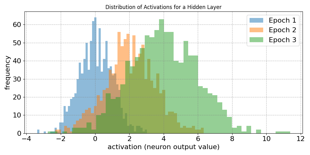
Notice that both the mean and variance of the distribution drifts over time (i.e., across epochs). This effect is independent from whether the training data was normalized or not. In other words, particularly in the context of deep neural networks, normalization issues reappear inside the network, even if the external input was well behaved.
Summary. In real-world data, unnormalized features are the norm because data is generated by heterogeneous processes. Different features often measure fundamentally different properties such as time, distance, money, or counts, using distinct units and conventions. This naturally leads to features with vastly different scales and orders of magnitude. From a data collection standpoint this is entirely reasonable, but for learning algorithms it means that raw numerical values are rarely directly comparable or equally informative. Unnormalized data also commonly appears in the form of incomparable units and distributions. Even when features have similar numeric ranges, they may encode entirely different semantics (e.g., temperature versus percentage), making their raw values misleading when combined in a model. In addition, many real-world quantities are highly skewed, with most observations concentrated near zero and a small number of extreme values dominating the range. Such skewness reflects underlying multiplicative or heavy-tailed processes and violates the assumptions of many models about linearity, symmetry, or constant variance.
Negative Effects of Unnormalized Data
Now that we know how unnormalized data may manifest itself in real-world datasets, let's have a look how this issue affect machine learning and data analysis methods etc. in practice. At the end of this section you should be convinced that the negative affects of unnormalized data can be seen across wide range of common methods.
Distance-based Methods
A large class of data mining and machine learning methods is built on the fundamental assumption that similar data samples should behave similarly. Rather than learning abstract rules alone, these methods explicitly compare samples to one another and base decisions on measured similarity or distance. This idea appears naturally in many real-world settings: users with similar preferences tend to like similar products, images with similar visual structure often depict the same objects, and documents with similar word usage usually discuss related topics. By grounding learning in pairwise relationships between samples, similarity-based methods provide an intuitive and flexible way to exploit structure in data without requiring strong parametric assumptions.
Some of the most popular algorithms in practice rely directly on this principle. Instance-based methods such as $k$-nearest neighbors classify or regress a new sample by examining the labels of its most similar neighbors. Clustering techniques, including hierarchical clustering, DBSCAN, and spectral clustering, define groups explicitly in terms of pairwise similarity or distance. Kernel-based methods, most notably support vector machines, encode similarity through kernel functions and express predictions as weighted combinations of similarities to selected training samples. In recommender systems, memory-based collaborative filtering operates almost entirely by comparing users or items and transferring information between those deemed similar.
Beyond these classical examples, similarity plays a central role in modern representation learning. Metric learning and contrastive approaches aim to learn a similarity function or embedding space in which semantically related samples are close together, forming the backbone of applications such as image retrieval, face recognition, and sentence similarity. Manifold learning methods like t-SNE and UMAP preserve local neighborhood similarities to uncover low-dimensional structure in high-dimensional data. Taken together, these approaches highlight that explicit sample-to-sample similarity is not a niche idea, but a unifying principle underlying many influential data mining and machine learning techniques.
To illustrate how different scales can affect similarity or distance-based methods, let's consider the following small dataset recording peoples' weight and height containing two label data samples and a third data sample for which we want to predict its class labels. Note that the weight of a person is recorded in kilograms (kg) and height in centimeters (cm) resulting both features being of similar scale.
| ID | Weight (kg) | Height (cm) | Class |
|---|---|---|---|
| A | 80 | 165 | 0 |
| B | 55 | 180 | 1 |
| C | 70 | 180 | ? |
Let's further assume we use a $k$-nearest neighbor (KNN) classifier with $k=1$ and use the Euclidean distance. To predict the class labels for Sample $C$, we need to compute the Euclidean distances $d_{euclidean}$ between $C$ and $A$, as well as between $C$ and $B$. The respective computations and the results (after some rounding) are as follows:
As the Euclidean distance between $C$ and $B$ is less than the Euclidean distance between $C$ and $A$, Sample $C$ is more similar to label $B$. The KKN classifier with $k=1$ would therefore label Sample $C$ as Class $1$.
Now let's change the dataset by changing the unit for height from centimeters (cm) to meters (m) as shown below. In other words, we change the values for feature "Height" by two orders of magnitude, making the scale now rather different compared to feature "Weight", which is still in kilogram (kg).
| ID | Weight (kg) | Height (m) | Class |
|---|---|---|---|
| A | 80 | 1.65 | 0 |
| B | 55 | 1.80 | 1 |
| C | 70 | 1.80 | ? |
If we compute the two Euclidean distances as before, we get the following results for this modified dataset:
With the height of a person given in meters (m), Sample $C$ is now more similar to Sample $C$, and our KNN classifier with $k=1$ would now predict Class $0$ for Sample $C$. In short, simply changing the unit of a feature caused the classifier to change its prediction. This is because the Euclidean distance — and many other distance or similarity metrics — is highly susceptible to the scale of individual features as it computes distance as the square root of the sum of squared feature-wise differences, causing features with larger numerical ranges to contribute disproportionately to the final distance. If one feature spans values in the hundreds (or more) while another may only vary only between $0$ and $10$, the larger-scale feature will dominate the distance computation, effectively drowning out the influence of smaller-scale but potentially informative features. As a result, similarity between samples becomes driven more by measurement units than by true semantic relevance.
Gradient-Based Optimization Methods
Unnormalized data is often problematic for gradient-descent-based methods because it creates ill-conditioned loss surface (or loss landscape), where different parameters experience gradients of vastly different magnitudes. When features have very different scales or distributions, the corresponding partial derivatives of the loss can differ by orders of magnitude. As a result, a single learning rate cannot be appropriate for all directions: steps that are small enough to keep training stable for large-scale features may be too small to make progress for small-scale ones, while steps large enough for small features can cause overshooting or divergence along large-scale directions.
This imbalance leads to loss surfaces that are elongated, skewed, or sharply curved in some directions and flat in others. Gradient descent then follows inefficient zig-zag trajectories, converges very slowly, or becomes numerically unstable. Highly skewed features and outliers further exacerbate the issue by producing gradients dominated by rare extreme values, pulling updates toward fitting those cases rather than the typical data. Normalization mitigates these problems by aligning feature scales and smoothing the geometry of the loss surface, making gradients more comparable and optimization more reliable.
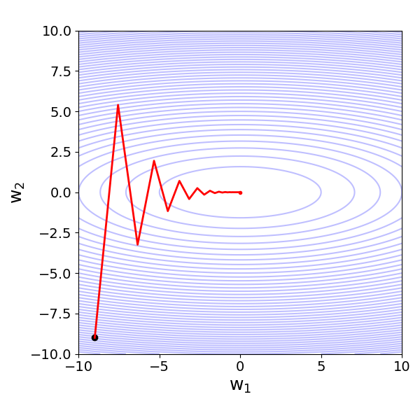
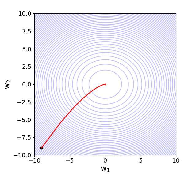
To visualize the problem, let's consider basic linear regression model with two input features $x_1$ and $x_2$ to predict an output value $y$; thus, our regression problem can be formulated as
where $\hat{y}$ is the prediction or estimate, $w_{0}$ is the bias terms (or offset), and $w_{1}$ and $w_{2}$ are the feature weights or feature coefficients. Ignoring the mathematical details, if we use the Mean Squared Error (MSE) as the loss function to be minimized using Gradient Descent — that is, finding the best values for all $w_{i}$ that minimize the loss — we get different loss surfaces depending on the difference of scale of both features $x_{1}$ and $x_{2}$.
For example, if the values of $x_2$ are about $100$ times larger than the ones of $x_1$, we get an ill-condition loss surface as shown in the left plot below. In this situation, the Gradient Descent algorithm would favor different loss functions with respect to the two weights/coefficients. However, since we have to rely on a single rate, we would need to balance between a slow convergence (low learning rate) and an inefficient zig-zag trajectory (high learning rate). In contrast, if both features are of (very) similar scale, the loss surface is much more well-behaved, where the gradients with respect to the different weights are also very similar. Here, a single learning rate works perfectly fine.
| $\large x_2 \sim 100\cdot x_1$ | $\large x_2 \sim x_1$ |
|---|---|
 |
 |
Variance-Based Methods
Many machine learning or data analysis algorithms rely on covariance, scatter, or similarity matrices. For example, Principal Component Analysis (PCA) Linear Discriminant Analysis (LDA), Factor Analysis (FA), Independent Component Analysis (ICA), and Canonical Correlation Analysis (CCA) all depend directly on variance and covariance estimates. If features have very different numerical scales, high-variance variables can dominate these matrices, biasing the learned directions or latent components toward large-scale features rather than truly informative structure. Similarly, methods such as Gaussian Mixture Models (GMMs) with full covariance matrices and spectral clustering rely on covariance estimation or distance-based similarities, both of which are strongly influenced by feature scale.
For a concrete example, lets consider Principal Component Analysis (PCA). PCA is a linear dimensionality reduction technique that transforms a dataset into a new coordinate system whose axes (called principal components) capture the directions of maximum variance. Instead of describing the data using the original features, PCA finds orthogonal (uncorrelated) directions along which the data varies the most. Mathematically, these directions are obtained as the eigenvectors of the covariance matrix, ordered by their corresponding eigenvalues (which measure how much variance each direction explains). In PCA, the first (largest) principal component is the direction in feature space along which the data exhibits the maximum variance. Intuitively, this direction captures where the data cloud is most spread out, meaning that projecting the data onto this axis preserves more information than any other single direction. All remaining principal components are chosen to be orthogonal to this first direction and explain progressively smaller amounts of variance.
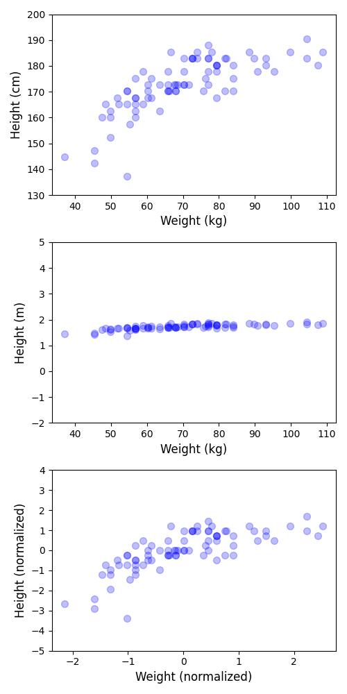
To give an example, let's consider a dataset containing the weight and height of 80 people, where the weight is measured in kilogram (kg) and the height in centimeters (cm). We can call this data roughly normalized since the values of both weight and are of a very similar scale. Now let's assume that we want to perform PCA to reduce the dimensionality of the dataset from $2$ to $1$. The figure below shows the results. The left plot shows the raw data points as well as the 1st principal component (i.e., the direction of the highest variance in the data); right shows shows the mapping from the $2$-dimensional space to the 1-dimensional space — consider that the transformed data points (dark blue) lie on a new x-axis.
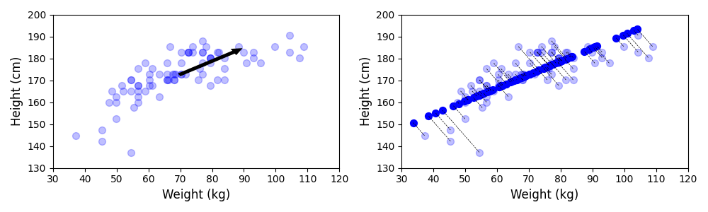
Like before, we can now modify the dataset by dividing all height values by $100$ so that the heights are now given in meters (m). Both features are now on rather different scales, with the weight values dominating the height values in absolute terms. This includes that the variance in weight is dominating the variance in height. Thus, if we now perform PCA on this modified dataset, we can clearly see how it changes the result; see the plot below showing the same two subplots as before.
In short, the output of any method that utilizes variances, covariances, scatters and so on will strongly depend on whether the data is normalized or not since it affects the variances of features and/or the covariances between features. Once again, we generally prefer features to be of similar scales to ensure that all features are considered of equal importance and no single feature will dominate the result.
Regularization Methods
A common sign that a parameterized model is overfitting is that some of its parameters (e.g., weights in a neural network or coefficients in a linear model) take on very large values. This often happens when the model tries to fit noise or other artifacts in the training data rather than capturing the underlying structure of the problem. Large parameter values allow the model to react strongly to small changes in input features, leading to highly complex decision functions that may perform extremely well on the training data but generalize poorly to unseen data.
This observation directly motivates the basic idea of regularization: explicitly encouraging parameters to remain small. By adding a penalty term that grows with the magnitude of the parameters, regularization constrains the model's flexibility and discourages extreme solutions that rely on large weights. As a result, the model is forced to explain the data using simpler, more stable patterns that are less sensitive to noise, thereby improving generalization and robustness without fundamentally changing the model architecture. Two common regularization methods a Lasso Regularizaion (least absolute shrinkage and selection operator) and Ridge Regularization; both regularization terms are defined as follows:
where $d$ is the number of parameters (e.g., weights or coefficients), and $\lambda$ is the regularization factor to regulate the importance of the regularization term. Those or similar regularization terms — we do not have to worry about their differences here — are added as some form of penalty to the loss function to encourage smaller parameter values during the training.
The important observation is that these penalties are applied uniformly to all coefficients, implicitly assuming that each feature contributes on a comparable scale. If the input features are not normalized, features with larger numerical scales tend to produce smaller coefficients (to achieve the same effect on the prediction), while features with smaller scales require larger coefficients. To quickly show this, consider a simple Linear Regression task with two input features — for example "Weight" and "Height" in the toy dataset above. This, for the $i$-the data sample, the regression equation for prediction $\hat{y}_i$ is:
If we would divide the values for feature $\mathbf{x}_2$ by 100 (e.g., to convert the values from centimeter to meter), to preserve the equation, we would need to multiply $w_2$ by 100 in return:
where $x^\prime_{i2} = x_{i2}/100$ and $w^\prime_{2} = w_{2}\cdot 100$. Since the scale of $w^\prime_{2}$ is now much larger, regularization would penalize $w^\prime_{2}$ much more. In short, As a result, the regularization penalty becomes uneven: it disproportionately penalizes features measured on smaller scales and under-penalizes those on larger scales, distorting the intended balance of the model.
Training Deep Neural Networks
As already seen, imbalanced gradients due to unnormalized input — either the initial input or as output from a previous layer — can pose challenges when it comes to gradient-based methods including the training of neural networks. More generally, neural network layers learn better when their inputs have similar, stable distributions, because gradient-based optimization assumes a reasonably well-behaved and consistent input space. If the distribution of inputs to a layer keeps changing, learning becomes unstable and inefficient. However, internal covariate shift may cause the distributions of activations to change during the training. One of the main reasons for this are the activation functions.
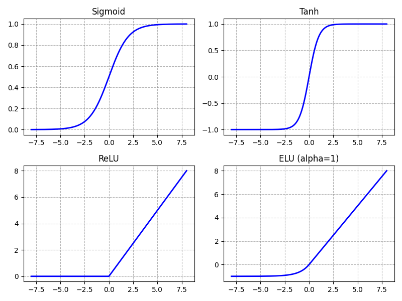
Neural networks rely on non-linear activation functions because, without them, a network with arbitrary many layers would collapse into a single linear transformation. Stacking linear operations only results in another linear function, which severely limits the types of relationships the model can represent. Many real-world problems involve complex, non-linear interactions between features, such as thresholds, hierarchies, or compositional patterns, that cannot be captured by linear models alone. The figure below plots $4$ popular activations as an.
Basically all common activation functions are scale-sensitive, which means that its output changes significantly when the scale (magnitude) of its input changes. In other words, multiplying the input by a constant factor can drastically alter the behavior of the activation, not just proportionally, but qualitatively. Internal covariate shift can negatively affect activations in two main but closely related ways:
Pre-activations outside the "healthy range": Activation functions such as Sigmoid or Tanh saturate when their input is very small or very large. For example, in the case of Sigmoid, only get "useful" gradients (i.e., gradients not close to $0$) between, say, $-5$ and $+5$; see the top-left plot in the figure above. Outside the range, the gradients become basically $0$. This is a problem since gradients of (close to) $0$ do not result in any meaningful training since parameters (i.e., weights and biases) are not updated. The phenomenon is also called vanishing gradients. Internal covariate shift can cause pre-activations to move outside this "healthy range".
Sensitivity of non-saturating activation functions: Even though activation functions like ReLU and ELU do not saturate for positive pre-activations, they can still be negatively affected by internal covariate shift. ReLU (bottom-left plot) is linear for positive inputs, but it is not symmetric and has a hard threshold at zero. If the distribution of pre-activations shifts even slightly, a large fraction of neurons may move from the positive (active) region into the negative (inactive) region. Since ReLU outputs exactly zero for negative inputs, this can suddenly shut off neurons and block gradient flow (the "dying ReLU" problem). ELU (bottom-right plot) mitigates this somewhat by allowing negative outputs instead of hard zeros, but it still has a nonlinear negative regime that can become saturated for sufficiently negative inputs. Moreover, activation functions that do not saturate for large positive or negative inputs carry a higher risk of contributing to exploding gradients because they do not inherently dampen the backpropagated signal. During backpropagation, gradients are multiplied layer by layer through activation derivatives and weight matrices. Non-saturating activations typically have derivatives close to a constant (e.g., $1$ for positive ReLU inputs), meaning they allow gradients to pass through largely unchanged. In deep networks or in the presence of large weights, this lack of attenuation can cause gradients to grow multiplicatively across layers, increasing the likelihood of exploding gradients.
The intuitive consequence of internal covariate shift is that each layer in a deep neural network must continuously adapt to a moving target: As earlier layers update their weights during training, the distribution of their outputs changes, which in turn changes the input distribution seen by subsequent layers. This means later layers cannot rely on a stable input distribution and must repeatedly readjust to shifting activation statistics. As a result, learning becomes slower and less stable, because layers are not only learning the task but also constantly compensating for changes introduced upstream. And again, this is still a common phenomenon even if the input data was properly normalized.
Common Normalization Strategies
Given the many potential negative effects of unnormalized data, the application of suitable normalization methods become very important to ensure meaningful results when analysing data or training machine learning models. In this section, we therefore outline some of the most common methods, but keep in mind that the following overview is not comprehensive.
External Normalization
External data normalization refers to preprocessing techniques applied to a dataset before it is fed into a machine learning model, where feature values are transformed using statistics computed from the training data (e.g., mean, standard deviation, min, max). The goal is to place features on comparable scales, reduce dominance of large-magnitude variables, and improve numerical stability and optimization behavior.
Scale-Based Normalization
Scale-based normalization refers to methods that adjust feature values using a measure of their dispersion (or scale) without necessarily centering them around zero. Instead of subtracting a mean or median, the feature is typically divided by a scale parameter such as the standard deviation, variance, maximum absolute value. The goal is to ensure that features have comparable magnitudes so that no single feature dominates distance computations or gradient updates. Common methods include:
- Min-Max Scaling (also called normalization to a fixed range) is a linear transformation that rescales a feature so that its minimum value becomes 0 and its maximum value becomes 1 (or more generally, to any chosen interval $[a,b]$. For a feature $x$, the transformation is
This preserves the relative distances between values but compresses or stretches them into a predefined range. Min–max scaling is particularly applicable when features have known and stable bounds, when preserving the original distribution shape is desirable. Its main advantages are simplicity, interpretability, and the fact that it preserves the original distribution’s shape (just rescaled). It also ensures all values lie within a controlled range, which can improve numerical stability. However, it is highly sensitive to outliers: extreme values determine the scaling range and can compress the majority of data into a narrow interval. Additionally, if new unseen data fall outside the original min–max range, the scaled values may exceed the intended bounds unless the scaling parameters are updated carefully.
- Standardization (also called z-score normalization) rescales a feature so that it has mean 0 and standard deviation 1. For a feature (x), the transformation is
where $\mu_x$ is the mean and $\sigma_x$ is the standard deviation of feature $x$. Unlike min–max scaling, standardization does not bound the data to a fixed interval; instead, it centers the distribution and expresses values in terms of how many standard deviations they deviate from the mean. It is particularly applicable when models assume or benefit from approximately zero-centered, comparable feature scales such as linear models, logistic regression, support vector machines, principal component analysis (PCA), and neural networks trained with gradient-based optimization. However, it is still affected by strong outliers because both the mean and standard deviation are not robust statistics. Additionally, since the transformed values are unbounded, extreme values can still occur, which may be undesirable in some applications.
- Median and IQR scaling (robust scaling) is a normalization technique that centers a feature by subtracting its median and scales it by dividing by its interquartile range (IQR), i.e., the difference between the 75th and 25th percentiles:
Because both the median and IQR are robust statistics, this method is particularly applicable when the data contain outliers or are heavily skewed. It is well suited for real-world datasets where extreme values are present but should not dominate the scaling process. However, it does not constrain the data to a fixed range, and if the underlying distribution is roughly normal without strong outliers, standardization may be more interpretable. Additionally, in very small datasets, percentile estimates (and thus the IQR) can be unstable.
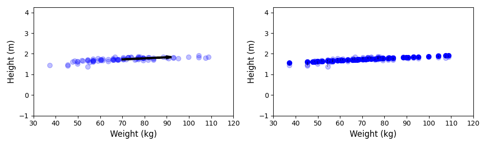
For an example, let's consider the same simple dataset containing the weights and heights of 80 people we have seen before. In the figure below, the plot on top shows the case where the weight is recorded in kilogram (kg) and the height in centimeters (cm), resulting in the two features of similar scale. The plot in the middle, in contrast, records the height in meters (m), in which case both features are on very different scales. The plot at the bottom shows the result after applying standardization to the dataset with kilogram and meter values (as seen in the middle plot).
Notice how the plot at them is again more similar to the plot at the top since the feature values are now normalized. The difference is of course the absolute scale — compared the ranges on the x-axis and the y-axis between both plots. After standardization, the weight and height values are no longer expressed in kilograms and meters but unit-free in terms of number of standard deviations away from the mean.
Distribution-Shaping Transformations
Distribution-shaping transformations are preprocessing techniques that modify the shape of a feature’s distribution to make it more symmetric, less skewed, or closer to a desired target distribution (often approximately normal). Unlike simple scaling methods that only adjust location or spread, these transformations change the functional form of the data. They are particularly useful when features exhibit heavy skew, long tails, or heteroscedasticity, which can negatively affect linear models, distance-based methods, or optimization procedures. The main benefit is improved statistical stability and better alignment with model assumptions, while a potential drawback is reduced interpretability, since the transformed values no longer correspond directly to the original measurement scale. Common transformation methods are:
Log transformation is a distribution-shaping technique in which each feature value $x$ is replaced by $\log(x)$ (commonly natural log or base-10 log). It is primarily used for positively skewed data, especially when values span several orders of magnitude (e.g., income, counts, or concentrations). By compressing large values more strongly than small ones, the log transformation reduces right skewness, stabilizes variance, and can make relationships more linear — properties that are beneficial for linear regression, generalized linear models, and other methods that assume homoscedasticity or approximate normality. When zeros are present, a shifted version such as $\log(x + c)$ (with $c > 0$) is often applied.
Power transformation is a family of distribution-shaping techniques that apply a parametric power function to a feature in order to reduce skewness and make the data more symmetric or approximately normal. Instead of using a fixed transformation like the logarithm, power transformations estimate an exponent parameter from the data. Common examples include the Box-Cox transformation (for strictly positive data) and the Yeo-Johnson transformation (which can handle zero and negative values). The main advantages are flexibility and data-driven adaptation: the transformation parameter is estimated to best normalize the distribution, often improving statistical efficiency and model performance. However, power transformations alter the original scale and interpretation of the data, can be sensitive to extreme outliers, and introduce an additional parameter-estimation step, which slightly increases preprocessing complexity.
Quantile transformation is a non-linear distribution-shaping technique that maps the original data to a target distribution (commonly uniform or normal) based on their empirical cumulative distribution function (CDF). Each value is replaced by its corresponding quantile and then mapped to the desired distribution, effectively reshaping the feature so that its output follows the specified distribution. The main advantage of quantile transformation is its strong ability to remove skewness and reduce the impact of outliers, since extreme values are mapped to extreme quantiles rather than dominating the scale. It can significantly improve model stability when distributional assumptions matter. However, it distorts the original distances between data points (because it is highly non-linear), which may negatively affect distance-based methods. It also depends on the empirical distribution of the training data, meaning that new unseen data may not align perfectly with the learned quantile mapping.
To illustrate the effect of a distribution-shaping transformation, consider a highly right-skewed data distribution of some feature $x$; see the left plot in the figure below. The plot on the right shows the distribution of the same feature of applying a log transformation, i.e., $\log{x}$.
After the log transformation, the distribution of the feature is very close to a normal distribution. Many statistical and machine learning methods assume or benefit from approximately normally distributed features because the normal distribution has convenient mathematical properties that simplify modeling, estimation, and inference. Normality often promotes balanced variance, reduced influence of extreme values, and more reliable statistical behavior.
Vector Normalization (Length-Based Scaling)
Vector normalization or length-based scaling is a technique that rescales a feature vector so that its overall length (or norm) equals a fixed value, typically 1. This approach is widely used in text mining, recommendation systems, and clustering, where the direction of the vector (relative proportions of features) matters more than its magnitude. The main difference compared to basic scale-based normalization like standardization is that vector normalization considers the vector as a whole and preserves relative proportions within the vector, whereas standardization rescales each feature independently to have zero mean and unit variance without controlling the overall vector length. The two most common vector normalization methods are:
- L2 normalization (or Euclidean norm scaling) is a type of vector normalization in which a feature vector $\mathbf{x}$ is rescaled so that its L2 norm (Euclidean length) equals $1$:
This ensures that all vectors lie on the unit hypersphere, preserving the relative proportions of features within each vector while standardizing overall magnitude. However, it does not account for the distribution of individual features across the dataset and may be less effective if feature scales vary widely or if absolute magnitudes carry meaningful information.
- L1 normalization (or called Manhattan norm scaling) rescales a feature vector $\mathbf{x}$ so that the sum of the absolute values of its components equals $1$:
This approach preserves the relative proportions of features within the vector while controlling its overall magnitude. The main advantages of L1 normalization are that it is robust for sparse data, ensures all vectors are comparable regardless of their original magnitude, and emphasizes the relative contribution of each feature. Unlike L2 normalization, it can produce more sparse representations and is less sensitive to very large individual components. However, L1 normalization may be less stable numerically if vectors contain many zeros, and it does not handle differences in feature scale across the dataset; extreme outliers in a single feature can still disproportionately influence the normalized vector.
The figure below, shows the example of $2$ documents represented by their document vectors (e.g., TF-IDF weight vectors) — the red and blue vectors in both plots. The black vector represents the vector of a search query. In the left plot, all vectors are unnormalized; notice the large difference between the red and blue document vectors. Assuming TF-IDF vectors, this difference in length is typically a strong indicator that the red vector represents a much longer document than the blue vector. Thus, if we would use the Euclidean Distance between the query vector and the document vector — illustrated by the dashedlined — the blue vector would be close to the query vector (left plot). However, in practice, we typically want to ignore the length of a document when it comes to computing the relevance of a document with respect to a query. The right plot therefore shows all $3$ vectors after L2 normalization, i.e., all vectors have length of $1$ (note that the scale of plot axes distort the length somewhat). After the normalization, the red vector is now closer to the query.
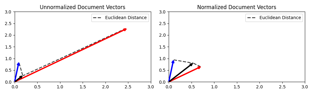
Side note: In practice, we typically use the Cosine similarity to compute the similarity between document vectors as it computes the angle between the vectors, which also is agnostic to the length of the vectors — because the Cosine similarity "internally" normalizes the similarity with respect to length of the vectors.
Internal Normalization
Internal normalization refers to normalization techniques that are applied inside a model during training, rather than preprocessing the input data beforehand. The term is most commonly used in the context of neural networks because deep networks consist of many stacked layers whose activation distributions continuously change during training ($\rightarrow$ internal covariate shift; see above). Instead of normalizing features once before feeding them into the model (external normalization), internal normalization adjusts the distributions of intermediate activations within the network itself. The goal is to keep layer inputs in a stable and well-behaved range (e.g., controlled mean and variance), which improves optimization, stabilizes gradients, and accelerates convergence.
While various internal normalization methods have been and are continuously being proposed, we focus on two of the most common methods: Batch Normalization and Layer Normalization, normalizing intermediate activations during training, thereby improving gradient flow and enabling deeper and more efficiently trainable networks. To illustrate the basic idea how both methods works, assume that the matrix below represent the output of a hidden linear layer of shape $\text{batch\_size}\times\text{num\_features}$ (here: $4\times 6$), where $\text{batch\_size}=4$ reflects the number of samples with the batch, and $\text{num\_features}$ reflects the number of features (i.e., the number of activations) of the hidden layer.
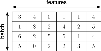
Let's see how Batch Normalization and layer normalization work based on these example activations.
Batch Normalization
Batch Normalization works by normalizing the activations of a layer using the statistics of the current mini-batch during training. For each feature (dimension) of the layer’s output, it computes the mini-batch mean and variance, subtracts the mean from each activation, and divides by the standard deviation (with a small constant added for numerical stability). This transforms the activations to have approximately zero mean and unit variance within that batch; see this step for our example output in the figure below.
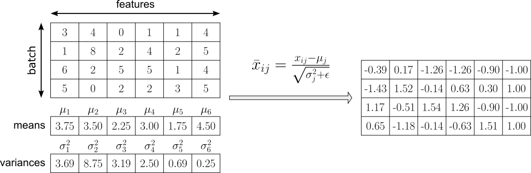
However, if the normalized activations were always forced to remain standardized, the layer would lose flexibility — some tasks may require activations to have a different scale or offset for optimal performance because strictly enforcing zero mean and unit variance could unnecessarily restrict the expressive power of the network. Batch Normalization therefore applies learnable parameters for each feature $j$: a scaling factor $\gamma_j$ and a shift parameter $\beta_j$. These allow the network to adjust the normalized values if a different distribution is beneficial for learning, ensuring that normalization does not reduce the model's expressive power. Thus, the final normalized activation $y_{ij}$ is computed as:
By adding $\gamma_j$ and $\beta_j$, the network can learn the most suitable distribution for each feature $j$, while still benefiting from stable normalization during optimization. In fact, if zero mean and unit variance were always optimal, the model could simply learn $\gamma_j=1$ and $\beta_j = 0$. However, in practice, different layers and features often benefit from different scales and biases. The learnable parameters ensure that normalization improves conditioning and gradient flow without limiting what the network can represent. In the extreme case, the layer could even learn to undo normalization if that were beneficial. After this normalization step, the method applies two During inference, instead of using batch statistics, Batch Normalization uses running (moving average) estimates of the mean and variance accumulated during training, providing stable and deterministic behavior.
Batch Normalization often leads to faster convergence and makes training deep networks more robust to weight initialization. Additionally, because normalization is computed over mini-batches, it introduces a small amount of stochastic noise, which can have a regularizing effect and sometimes reduces the need for other techniques like dropout. However, its reliance on mini-batch statistics makes it sensitive to small batch sizes, where estimated means and variances become noisy and unstable. It also introduces a discrepancy between training (using batch statistics) and inference (using running averages), which can slightly complicate deployment. Furthermore, it is less well-suited for certain architectures such as recurrent neural networks or very small-batch settings, where alternative normalization methods (e.g., layer normalization) may perform better.
Layer Normalization
In contrast to Batch Normalization, Layer Normalization works by normalizing the activations of a single data sample across its feature dimensions, rather than across the batch. For each individual example, it computes the mean and variance over all features in a given layer, then subtracts the mean and divides by the standard deviation (with a small constant added for numerical stability); see this step for our example output in the figure below.
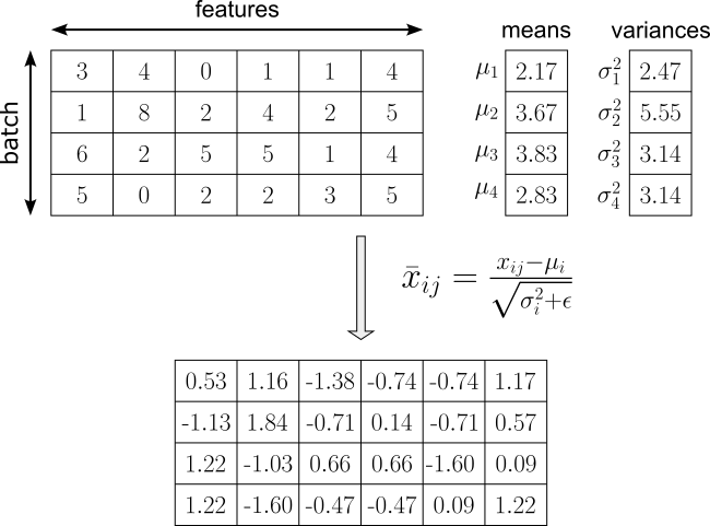
Since each sample has again zero mean and unit variance, Layer Normalization also introduces learnable scaling and shifting parameters. In fact, the learnable scaling parameters are still defined per feature dimension (not per sample) — the same way as for Batch Normalization. Thus, there is again one $\gamma_j$ and one $\beta_j$ for each feature $j$, shared across all samples, resulting the the same formula:
The key advantage of Layer Normalization is that it does not depend on mini-batch statistics. Because normalization is performed independently for each sample across its feature dimensions, it works reliably with small batch sizes and even batch size 1. It also behaves identically during training and inference, avoiding discrepancies between batch statistics and running averages. This makes it particularly well-suited for sequence models such as recurrent neural networks and transformer architectures, where batch sizes may vary or temporal dependencies make batch-wise normalization less appropriate. On the flip side, Layer Normalization does not benefit from the regularizing effect that arises from noisy batch statistics in Batch Normalization. It may also be less effective in convolutional neural networks, where feature-wise normalization across spatial dimensions can sometimes better exploit the structure of image data. In practice, while it improves training stability, it often does not accelerate convergence in feedforward or convolutional networks as strongly as batch normalization does.
Alternative Methods
Besides Batch Normalization and Layer Normalization, several other internal normalization methods are commonly used, often tailored to specific architectures. Here is a brief outline
Instance Normalization: Primarily used in convolutional neural networks (CNNs), especially in image generation and style transfer. It normalizes each sample and each channel independently across spatial dimensions, making it effective for removing instance-specific contrast information.
Group Normalization: Designed mainly for CNNs when batch sizes are small. It divides channels into groups and normalizes within each group across spatial dimensions. It provides more stable behavior than Batch Normalization in small-batch settings and is widely used in object detection and segmentation models.
Weight Normalization: Instead of normalizing activations, it reparameterizes weight vectors to decouple their magnitude and direction. It is applicable to fully connected and convolutional layers and is sometimes used in recurrent networks to improve optimization without relying on batch statistics.
Spectral Normalization: Commonly used in generative adversarial networks (GANs). It constrains the spectral norm (largest singular value) of weight matrices to stabilize training and control Lipschitz continuity, particularly in discriminator networks.
RMS Normalization: A simplified variant of Layer Normalization that normalizes using only the root mean square (without subtracting the mean). It is frequently used in large transformer architectures because it reduces computational overhead while maintaining training stability.
The choice of normalization method strongly depends on architecture and batch size: CNNs often use Batch, Group, or Instance Normalization; recurrent networks and transformers typically rely on Layer Normalization or RMS Normalization; and generative models like GANs may additionally use Spectral Normalization for stability.
Summary
In real-world datasets, it is very common to encounter unnormalized data, where different features have vastly different scales, units, or ranges. The presence of unnormalized data can have several negative consequences in data analysis and machine learning. For similarity-based methods such as k-nearest neighbors or clustering, large-scale features dominate distance calculations, distorting the notion of "similarity" between samples. In machine learning models, especially gradient-based models like neural networks, unnormalized features can slow down convergence, cause unstable gradients, or lead to poor generalization. Even statistical methods such as principal component analysis (PCA) can be heavily skewed, as features with larger variances dominate the principal components, masking the contributions of smaller-scale but meaningful features.
To address these issues, data normalization strategies are employed to transform features into comparable scales or distributions. One broad approach is scale-based normalization, which adjusts features to a fixed range or magnitude. Another category is length-based or vector normalization, which scales each data point such that its feature vector has a unit norm. Normalization can also be applied internally within machine learning models, for example through batch normalization or layer normalization. These approaches stabilize the training of deep networks by keeping intermediate activations in well-conditioned ranges, mitigating issues like internal covariate shift. Overall, normalization is a crucial preprocessing step that ensures fair feature contributions, stabilizes model training, and improves the quality of data-driven analyses.
A solid understanding of unnormalized data and normalization strategies is essential because many analytical and machine learning methods implicitly assume that features are comparable in scale and distribution. When this assumption is violated, results can become misleading: distance-based methods may overemphasize large-scale variables, optimization algorithms may converge slowly or unstably, and model parameters may become difficult to interpret. Without recognizing the presence and impact of unnormalized data, practitioners risk attributing poor performance to the wrong causes rather than to basic data representation issues.
Moreover, choosing an appropriate normalization strategy is not merely a technical detail but a modeling decision that directly influences learning dynamics and generalization. Different techniques (including standardization, min-max scaling, vector normalization, or internal normalization within neural networks) serve different purposes and make different assumptions about the data. Understanding these distinctions enables informed decisions about when and how to normalize, leading to more robust analyses, faster training, and more reliable conclusions.