Disclaimer: This Jupyter Notebook contains content generated with the assistance of AI. While every effort has been made to review and validate the outputs, users should independently verify critical information before relying on it. The SELENE notebook repository is constantly evolving. We recommend downloading or pulling the latest version of this notebook from Github.
Decision Trees
Decision Trees are one of the most intuitive and widely used machine learning algorithms for both classification and regression tasks. At their core, decision trees represent a flowchart-like structure, where data is split recursively based on certain conditions until a final decision or prediction is made. Each internal node of the tree corresponds to a decision or test on a feature, each branch represents the outcome of the test, and each leaf node signifies a final prediction or category. Their hierarchical nature makes decision trees easy to visualize and interpret, making them highly suitable for both beginners in machine learning and professionals seeking explainable AI models. The versatility of decision trees allows them to excel in a range of applications, including but not limited to, medical diagnosis, customer segmentation, fraud detection, and predictive maintenance. For example, a decision tree might help a doctor determine whether a patient has a particular disease by analyzing their symptoms step-by-step. Similarly, businesses use decision trees to classify customer behavior and tailor marketing strategies. Their ability to handle both categorical and continuous data makes them a robust choice for solving real-world problems.
Learning about decision trees is crucial for several reasons. First, they provide a foundational understanding of how data-driven decisions are made, which is essential for grasping more advanced algorithms like Random Forests and Gradient Boosting Machines. Second, decision trees are inherently interpretable, making them ideal for scenarios where transparency is necessary, such as in healthcare or legal domains. Finally, their simplicity and efficiency in handling both small and large datasets make them a fundamental tool in any data scientist's toolbox. In addition, decision trees play a pivotal role in ensemble learning methods, where multiple decision trees are combined to create more robust and accurate models. Algorithms like Random Forests and XGBoost rely on decision trees as their building blocks, showcasing their importance even in advanced machine learning techniques. By understanding the principles of decision trees, one can better comprehend and implement these powerful ensemble methods.
Setting up the Notebook
Make Required Imports
This notebook requires the import of different Python packages but also additional Python modules that are part of the repository. If a package is missing, use your preferred package manager (e.g., conda or pip) to install it. If the code cell below runs with any errors, all required packages and modules have successfully been imported.
import pandas as pd
from src.utils.data.files import *
Download Required Data
Some code examples in this notebook use data that first need to be downloaded by running the code cell below. If this code cell throws any error, please check the configuration file config.yaml if the URL for downloading datasets is up to date and matches the one on Github. If not, simply download or pull the latest version from Github.
bank_data ,_ = download_dataset("tabular/classification/example-credit-default-data.csv")
File 'data/datasets/tabular/classification/example-credit-default-data.csv' already exists (use 'overwrite=True' to overwrite it).
Basic Idea
Example Application
Banks give out credit as a fundamental part of their business model to earn profits and facilitate economic activity. By extending credit in the form of loans, mortgages, or credit cards, banks generate revenue through the interest charged on the borrowed amount. This interest is a primary source of income for banks, enabling them to cover operational costs, pay interest to depositors, and provide returns to shareholders. Offering credit also helps banks attract customers and build long-term relationships, which can lead to cross-selling of other financial products like insurance, investment services, or savings accounts. Issues arise when a bank customer "defaults" on their credit, which means they have failed to meet the repayment obligations outlined in their credit agreement. Consequences for the bank include not only financial losses but also operation costs (costs are associated with attempting to collect the debt or writing it off), and increased risk reserves (the bank must allocate more capital to cover potential future losses, which affects its profitability and lending capacity).
Therefore, banks try to predict whether a customer will default on their credit to manage risks effectively and ensure financial stability. Predicting defaults allows banks to identify high-risk customers in advance and take preventive measures, such as adjusting credit limits, requiring collateral, or offering stricter terms for repayment. This risk assessment ensures that the bank minimizes potential losses while continuing to lend profitably. Moreover, predicting credit defaults is crucial for compliance with regulatory requirements. Financial institutions are often required to maintain adequate capital reserves to cover potential losses from defaults. By accurately predicting which customers are likely to default, banks can allocate these reserves more effectively and ensure they meet regulatory standards. This not only helps maintain trust in the banking system but also contributes to overall economic stability. Predicting defaults also enhances customer management, as banks can proactively engage with at-risk customers to explore solutions like debt restructuring or financial counseling, benefiting both parties.
In the following, we play the bank and use a very simple example dataset of customers' information and whether they defaulted on their credit or not. The dataset contains the credit application record for only nine customers, with each customer describe by four attributes: Age, Education (Bachelor, Masters, or PhD), Martial_Status (Single or Married), and Annual_Income. The attribute Credit_Default (Yes or No) indicates if the customer defaulted on their credit or not. Let's load the data from the file into a pandas DataFrame and have a look:
df_bank = pd.read_csv(bank_data)

df_bank.head(10)
| ID | Age | Education | Marital_Status | Annual_Income | Credit_Default | |
|---|---|---|---|---|---|---|
| 0 | 1 | 23 | Masters | Single | 75000 | NO |
| 1 | 2 | 35 | Bachelor | Married | 50000 | YES |
| 2 | 3 | 26 | Masters | Single | 70000 | NO |
| 3 | 4 | 41 | PhD | Single | 95000 | NO |
| 4 | 5 | 18 | Bachelor | Single | 40000 | YES |
| 5 | 6 | 55 | Masters | Married | 85000 | YES |
| 6 | 7 | 30 | Bachelor | Single | 60000 | YES |
| 7 | 8 | 35 | PhD | Married | 60000 | NO |
| 8 | 9 | 28 | PhD | Married | 60000 | NO |
For example, the customer with ID 1 was 23 years of age, had a Master's degree, was single, had an annual income of $75,000, and did not default on their credit.
Rule-Based Classification
Now assume we want to find some rules that could tell us if new customers are likely to default on their credit based on this historical dataset. If the result would say "YES" then we might consider not approving their credit (or adjusting credit limits, requiring collateral, or offering stricter terms for repayment). Just by looking at this data set, you might notice some patterns, for example:
- All customers that were single and earned more than $S65k did not default on their credit
- All customers with a Master's degree and older than 50 did default on their credit
- ...
The goal is to find a rule set that correctly captures all customers in our dataset. If we would take some time and try different combinations of conditions, we might come up with the following rule set in pseudo code:
IF Marital_Status IS "Single" THEN
    IF Annual_Income < 65000 THEN
        RETURN "YES"
    ELSE
        RETURN "NO"
    END IF
ELSE
    IF Education IS "PhD" THEN
        RETURN "NO"
    ELSE
        RETURN "YES"
    END IF
END IF
You can try each customer in the dataset to convince yourself that the rule set indeed matches a customer to the recorded output. In fact, we can quickly implement this rule set by transforming the previous pseudo code into a Python method that takes the four relevant attributes as input and returns either "YES" or "NO" for the predicted Credit_Default attribute. Notice that we call the method predict_default_v1() since we will later implement a second predict method accomplishing the same task.
def predict_default_v1(age, education, marital_status, annual_income):
    if marital_status == "Single":
        if annual_income < 65000:
            return "YES"
        else:
            return "NO"
    else:
        if education == "PhD":
            return "NO"
        else:
            return "YES"
We can now iterate over all entries in our customer dataset to predict if the customer would default on their credit using the methods predict_default_v1().
for idx, row in df_bank.iterrows():
    prediction = predict_default_v1(row["Age"], row["Education"], row["Marital_Status"], row["Annual_Income"])
    print(f"[ID {idx+1}] {prediction}")
[ID 1] NO
[ID 2] YES
[ID 3] NO
[ID 4] NO
[ID 5] YES
[ID 6] YES
[ID 7] YES
[ID 8] NO
[ID 9] NO
The predicted results should match the values in the Credit_Default column in the original dataset.
Decision Tree
If you look at the pseudo or Python code, you will notice that the rule set is implemented using nested if...else statements with each condition introducing a conditional branch. Such a branching structure can be graphically represented by a tree, giving us our basic idea of a Decision Tree. The figure below shows the Decision Tree reflecting the rule set we defined above.
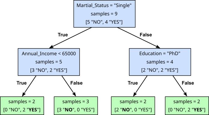
A Decision Tree has three main components:
Internal nodes: An internal node in a Decision Tree — a blue box in the figure above — refers to a node that represents a decision point where the data is split based on a certain feature's value. Each internal node typically contains (a) a condition based on a feature's threshold (e.g., Annual_Income < 65,000?), (b) the number of $samples$ from the training that have reached that node, and (c) the distribution of class labels
Branches: a branch represents outcome of a condition of an internal node and corresponds to a feature (e.g., Education ="PhD") value or range of values (e.g., Annual_Income < 65,000?). Depending on the condition of an internal node, the inner node may have two or more outgoing branches. In the example Decision Tree above, each internal node yields only two branches; however, this is not a fundamental requirement.
Leaf nodes: A leaf node in a Decision Tree — a green box in the figure above — represents the end point of a decision path, where no further splitting occurs. It contains the final output or prediction for the data that reaches it. In classification tasks, a leaf node typically holds the most common class label of the data points that have traversed the path to that node. In regression tasks, it stores the average or mean value of the target variable for the data that reaches the leaf. In the example above, each leaf only contains samples from a single class; again, this is not a fundamental requirement.
Once we have such a Decision Tree, we can use it to make predictions on new unseen data. For example, consider a new customer (50, PhD, Single, $70,000) applying for a credit. Based on our training data of historical information, do we believe this customer will default on their credit? According to the root not of the Decision Tree, we first need to check if the customer is Single or Married. Since the customer's marital status is Single, we follow the left branch of the root node. This brings us to the internal node requiring us to check if the customer's annual income is below $65,000. This is not the case, so we follow the right branch. This brings us to a leaf node which means we can make our prediction. As the majority class label — and in fact the only class label — in this leaf node is "NO", we predict that the customer will not default on their credit. We can confirm this using our method predict_default_v1() that implements this simple series of tests:
print(predict_default_v1(50, "PhD", "Single", 70000))
NO
Training Decision Trees
The example banking dataset containing information if customers have defaulted on their credit was small and simple enough — only nine samples and four attributes — that we could find a working Decision Tree just looking "long and hard" enough at data. Of course, in practice, training datasets are much larger containing hundreds of thousands data samples and maybe hundreds of attributes. We therefore need an automated way to learn a Decision Tree from data. Before we delve deeper into different Decision Tree learning algorithms, it is important to highlight two observations.
Multiple Possible Decision Trees
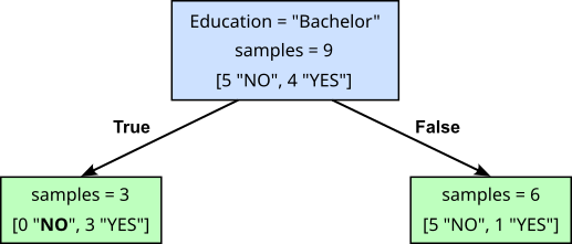
For any given training dataset, there is generally never a single Decision Tree that maps each sample to its output (class label or regression value) based on the sample's attributes. Particularly if the number of tests — the internal nodes in the Decision Tree or the if...else statements in a naive implementation does not matter — it is easy to convince yourself that one can always come up with more fine-grained rules. This is particularly true for large datasets, but also for small datasets there are typically multiple Decision Trees that match a given training dataset. For example, for out bank dataset, the following Decision Tree also maps each customer record to the correct label "YES" or "NO":

Naturally, we can directly implement this code as another prediction method, this time called predict_default_v2().
def predict_default_v2(age, education, marital_status, annual_income):
    if education == "Bachelor":
        return "YES"
    else:
        if age < 50:
            return "NO"
        else:
            return "YES"
And we can double-check again if this method works correctly by predicting the class label for each training sample.
for idx, row in df_bank.iterrows():
    prediction = predict_default_v2(row["Age"], row["Education"], row["Marital_Status"], row["Annual_Income"])
    print(f"[ID {idx+1}] {prediction}")
[ID 1] NO
[ID 2] YES
[ID 3] NO
[ID 4] NO
[ID 5] YES
[ID 6] YES
[ID 7] YES
[ID 8] NO
[ID 9] NO
Once again, we get the expected prediction as given by the training data. This means that both predict_default_v1() and predict_default_v2() make the same prediction with respect to the training data. This, in turn, means that both Decision Trees are possible solutions for our training data. While the two trees — and there are more! — look different, the important observation is that different trees may yield different predictions for unseen data. For example, consider the same new customer (50, PhD, Single, $70,000) applying for a credit. We can now use both auxiliary methods the implement our Decision Tree to make a prediction:
print(predict_default_v1(50, "PhD", "Single", 70000))
print(predict_default_v2(50, "PhD", "Single", 70000))
NO
YES
For this customer, both Decision Trees make different predictions. Or more generally, two Decision Trees that perform the same on the training dataset, may perform very differently on a test dataset. This implies that some Decision Trees are better than others with respect to some test data. In other words, we are not looking for only a Decision Tree but ideally for the best Decision Tree for a particular task and dataset.
Complexity of Problem
Although we would like to find the best Decision Tree, it turns out that this problem is in fact NP-hard. In simple terms, a problem is NP-hard if there is no efficient algorithm — that is, an algorithm with a polynomial runtime — that will solve that problem. The problem of finding the best Decision Tree for a dataset is NP-hard because it involves searching through an exponentially large space of possible trees to identify the one that best fits the test data. The key reasons are:
Exponential search space: For a given dataset, there are numerous ways to split the data at each internal node based on different features and thresholds. At each level of the tree, the algorithm must evaluate many possible feature thresholds and split points, which leads to an exponential growth in the number of possible Decision Trees as the dataset size and number of features increase.
Combinatorial nature: The Decision Tree construction process requires selecting the best feature and threshold at each node, and this decision impacts the structure of the tree. To evaluate all possible combinations of splits across all nodes and features requires checking an enormous number of configurations, which is inherently combinatorial. As a result, no known algorithm can solve this problem in polynomial time, thus making it NP-hard.
Summing up, this observation makes exhaustive search impractical for large datasets, which is why any practical implementations of Decision Tree learning algorithms rely on heuristics and greedy algorithms, as they provide near-optimal solutions in much less time. While the resulting Decision Trees are very likely to be good solutions, we have to keep in mind that they are not guaranteed to be the best solutions.
Building a Decision Tree — Core Concepts
There are several important learning algorithms for Decision Trees — and we cover the most popular ones later — but they all share fundamental concepts that derive from the tree structure of the model. In the following, we go through the concepts on an abstract level and outline how different Decision Learning algorithms handle them.
Basic Construction Process
All Decision Tree learning algorithms follow a top-down approach. When building a Decision Tree, we start with a single root node which contains the entire dataset. For our banking dataset, the root node looks as follows:
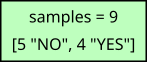
Since we do not test any condition that would lead to any branching, our single root node is a leaf node. In principle, we could stop here and use this "tree" to make predictions. In case a leaf node contains samples from multiple classes, the majority class is commonly used as the prediction. In other words, we would always predict "NO" for any training or test sample, independent from its feature values. This is arguably not a very useful model. To make more meaningful predictions that take the features of samples into account, we need to start splitting nodes.
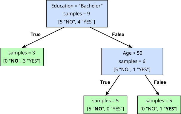
Splitting a current leaf node means that the algorithm selects the best feature and threshold (based on some criterion) to split the dataset into smaller subsets. How the best split is determined depends on the specific Decision Tree learning algorithm. For now, let's assume that we have some oracle that tells how to split a leaf node. For example, for our banking dataset, let's assume that the oracle tells us that we should split the root node by check Education of a customer is "Bachelor" or not. This will result in the following split:
Our root node has now become an internal node as it contains a test on a feature resulting in two branches ending in two new leaf nodes. In our small dataset, there are customers with a "Bachelor" degree. For these three customers, the split condition is true. Thus, the corresponding three data samples move to the left child node (the "True" branch); all remaining six samples (with a "Masters" or "PhD" degree) move to the right child node (the "False" branch).
If we would stop the construction process here, our Decision Tree would already perform fairly well. Assuming we always use the majority class label to make predictions, we would only misclassify only one sample from our training dataset. More specifically, we would misclassify the sample with ID 6 representing the customer (55, Masters, Married, $85,000). This customer has defaulted on their credit but we would predict "NO" with the Decision Tree above. However, this is not necessarily a bad thing. Maybe this sample is an outlier we should ignore. This idea will later bring us to the concept of pruning and similar strategies to handle the risk of overfitting with Decision Trees. Right now, let's assume we want to find a tree where all leaves contain only samples of a single class label.
When looking at our current Decision Tree, we can see that we have already achieved this goal for the left leaf node. All three samples contained in this leaf node have the same class label "NO". There is therefore no need for further splitting this node. In contrast, the right leaf node still contains samples of both classes. Hence, we recursively continue the same splitting process by finding the best split for this leaf node. As before, we ask our oracle and it tells us that we should now check if the Age if the customer was below $50$ or not. Splitting the leaf node based on this condition will again turn this node into an internal node with to branches pointing two new leaf nodes:
In short, Decision Trees grow by recursively checking all leaf nodes if a split is required and, if so, perform the split. By default, we can stop splitting a leaf node if it only contains samples of the same class label — or just a single data sample, which is just a special case of the former condition. In practice, the process of splitting may stop before these bases cases if some other predefined stopping criteria is satisfied. For example, we may want to specify that a Decision Tree should not exceed a maximum depth, or that a leaf node has to contain a minimum number of samples. Again, a deeper discussion of such criteria and their purpose is beyond the scope here.
If we check both new leaf nodes that were added after the last split, we can see that both satisfy the default stop condition, since both leaf nodes only contain samples of the same class — only "NO" in the left child node and only "YES" in the right child node. Thus, the learning algorithm stops and we have trained our final Decision Tree. Of course, for large datasets, the resulting Decision Tree is likely to be much larger with many more internal and leaf nodes. However, the process of recursively splitting leaf nodes until some stopping criterion is satisfied remains exactly the same.
As long as the training data does not contain ambiguous data, we can also construct a Decision Tree where each leaf contains only samples of the same class. Ambiguous data refers to the situation where two or samples have the same feature values but different class labels, for example:
| ID | Age | Education | Marital_Status | Annual_Income | Credit Default |
|---|---|---|---|---|---|
| ... | ... | ... | ... | ... | ... |
| 6 | 55 | Masters | Married | 85,000 | YES |
| ... | ... | ... | ... | ... | ... |
| 102 | 55 | Masters | Married | 85,000 | NO |
| ... | ... | ... | ... | ... | ... |
In general, this means the available features themselves are insufficient to distinguish between classes, which can be quite common in many applications. For example, in our banking use case, it is not unlikely that two customers may have the same features, but one has defaulted in their credit while the other has not. Such label conflicts will prevent achieving a pure split, leaving leaf nodes with mixed class labels. However, label conflicts due to ambiguous data are a general challenge and not limited to Decision Trees but affect all machine learning models.
All popular Decision Tree learning algorithms follow this top-down strategy of starting with a single root node and recursively splitting leaf nodes. The key advantages of strategy are:
Simplicity and intuitiveness: The top-down approach mirrors how humans often solve problems: starting broadly and refining decisions step-by-step. It provides a straightforward, systematic method for tree construction.
Greedy optimization: The algorithm uses a greedy approach at each node, choosing the split that optimizes a specific criterion (discussed later) for that step. This localized optimization is computationally efficient and reduces the need for complex global optimization techniques.
Efficiency and scalability: The top-down approach is computationally efficient, as it processes one level at a time. Since it does not require backtracking, it avoids the overhead of revisiting earlier splits to check their validity or improve them. It can handle large datasets effectively because it progressively reduces the size of subsets at each level. Each split reduces the number of data points considered for the next level, making the process manageable.
Modularity: The recursive nature of the top-down approach allows for modular implementation. Each node can be treated as an independent problem, enabling easier debugging and parallelization in some cases.
Interpretability: The decisions made at each step are based on well-defined criteria (e.g., splitting on the most informative feature). This step-by-step logic makes the resulting decision tree easy to interpret and explain.
Adaptability: The algorithm can adapt to different problems and datasets by tweaking the splitting criteria or stopping conditions (e.g., maximum depth, minimum samples per leaf). Different types of top-down decision tree algorithms can be tailored to suit specific tasks, such as classification or regression.
Compatibility with pruning: A tree generated using a top-down approach can be pruned afterward to improve generalization and prevent overfitting. Pruning methods like reduced-error pruning or cost-complexity pruning complement the top-down construction process.
While the top-down approach has many advantages, it also has limitations. Most importantly, it may not find the globally optimal tree because it makes greedy decisions at each step without considering the overall structure. It can overfit noisy or imbalanced data if stopping criteria or pruning are not applied effectively. Despite these limitations, the top-down approach remains one of the most practical and widely used methods for decision tree learning.
Finding the Best Split
When covering the basic top-down strategy for constructing a Decision Tree, we skipped over the task of how to split a leaf node (if necessary). So far, we assumed to have some oracle that tells which condition to use to split the dataset into child nodes. Of course, in practice, such an oracle is not available. Therefore, a Decision Tree learning algorithm has to programmatically find the most suitable condition to split a node. While this is a task where most learning algorithms differ from each other with respect to the exact implementation, the general criterion is the same. Recall that, by default, we stop training a Decision Tree if all leaf nodes contain only samples of the same class. Intuitively, this means that we prefer splits that better separate data samples with respect to their class labels.
To illustrate this, let's look again at the root node of our banking dataset:
For splitting this node, we not only to choose between any of the four inputs features (Age, Education, Martial_Status, Annual_Income), but for the selected feature we also have to choose a threshold — or more since, in general, a split may yield more than two branches. From all those possible, let's just look at two of them. In fact, there are the to roots splits we saw in the previous example:
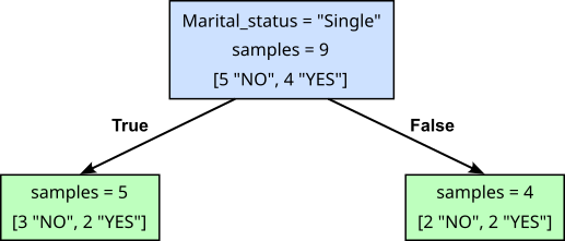
We saw that both root split yield Decision Trees mapping the samples from the training data to their respective class labels with respect to the samples' feature values. So the question is: Which split do we consider the preferred choice? The rationale of all Decision Trees is that they prefer splits that result in a better separation of the data samples according to their classes. Before the split, we start with a leaf node with a fairly mixed set of class labels (5 "NO" and 4 "YES"). Splitting this node based on condition if the Marital_Status of a customer is "Single", we end up with to child nodes where the class labels are still very much mixed (3 "NO" and 2 "YES" in the left child node; 2 "NO" and 2 "YES" in the right child node). In simple terms, we didn't really make much progress.
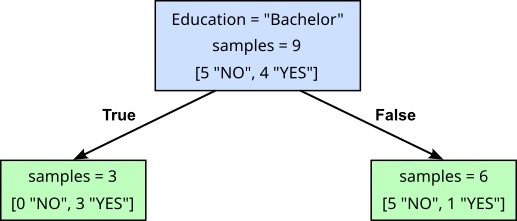
In contrast, when splitting based on the condition of a customer has a "Bachelor" degree, the class labels in the child nodes are much more separated. In fact, the left child node contains only samples of class "NO", so no further splitting required here. But also the right child node is already quite separated with only 1 "YES" beside 5 "NO". This means, given these two choices to split the root node, we prefer the second split based on customers "Education". For any practical implementation of a Decision Tree Learning algorithm, we need a way to quantify if a split yields a better or worse separation of class labels. And different learning algorithms use different metrics.
Still, keep in mind that this approach is only a heuristic since the decision which split is preferred is a "local" decision that only depends on the current leaf node in question. This decision does not incorporate any future splits. For example, splitting our root nodes based on customers "Martial_Status" might seem suboptimal when it comes to separating the class labels, but subsequent split may result in a final Decision Tree that performs better than the one using "Education" for the split condition in the root node.
Learning Algorithms for Decision Trees — Overview
We now have a basic understanding of what Decision Trees are and how we can train them for a given dataset. However, the exact process of training a Decision tree depends on the task (classification or regression), the type of data (numerical or categorical), the splitting criteria, and other characteristics. As such, there are a range of popular Decision Tree learning algorithms that differ in their application to accommodate different tasks and types of data, support different splitting criteria, may handle missing values, and so on. To wrap up this introductory notebook, we briefly discuss the main characteristics and provide a brief outline of the most popular Decision tree learning algorithms.
Characteristics
Support Tasks
Decision Trees supervised machine learning models. However, not all Decision Tree learning algorithms can be used for all tasks. Among the most popular learning algorithms ID3, C4.5/C5.0, and CHAID are suitable for classification tasks. In contrast, M5 can only be applied to regression tasks. CART can be used for both classification and regression tasks.
Type of Data
In principle, Decision Trees can be trained using numerical and/or categorical data; as we have seen in our small banking use case. However, not all learning algorithms actually support both types of data. For example, the native implementations of CART and M5 assume numerical data, while the native implementations of ID3 and CHAID assume categorical data. Of course, we can preprocess the data using
- Encoding (or continuization) to transform categorical data into numerical data
- Discretization to transform numerical data into categorical data.
Such steps are particularly important if a dataset contains both numerical and categorical features, just like our banking dataset. For example, without first somehow encoding Education and Marital_Status as numerical features, we would not be able to directly use the Decision Tree implementation of the scikit-learn library, since this implementation is based on the CART learning algorithm. For example, we could use binary encoding the converted the values for Martial_Status from "Single" and "Married" to $0$ and $1$. If we assume the the values for "Education" have a natural order, we can use ordinal encoding to convert the values as follows: "Bachelor" $\rightarrow 0$, "Masters" $\rightarrow 1$, and "Bachelor" $\rightarrow 1$. After those transformation steps all four customer features are numerical allowing to train a Decision Tree using the, for example, CART learning algorithm.
Splitting Criteria
As mentioned previously, all Decision Tree Learning algorithms split a node to effectively separate the class labels (in case of classification task). In other words, the overall goal is to find splits that minimize the "impurity" of the child nodes, where impurity reflects how many samples of different classes a node contains. For example, a node is considered "pure" if all samples in the node are of the same class. In contrast, if all classes appear equally frequent the node is very "impure". In a nutshell, different algorithms use different means to measure the impurity of nodes and/or the decrease of impurity caused by a split to find the best split. Without going into detail here, the most common metrics are:
- Entropy and entropy-based criteria
- Gini impurity
- Variance reduction (for regression tasks)
While the formula behind the different metrics might vary, their effects can be very similar; after all, they all have the same overall goal. For example, the CART algorithm works with both Entropy and Gini Impurity, and it has been shown that it makes no difference in almost all cases.
Handling Missing Data
So far, we assume that the dataset for training a Decision Trees has no missing values. Unfortunately, missing values are common in real-world data. For example, in our banking dataset, we might not have the Education level for all customers, or unemployed customers cannot report an annual income. In general, handling missing values is a common data preprocessing step since most machine learning algorithms cannot handle missing values and will throw errors. Without going into details common strategies include to simply remove data samples with missing values, or imputation techniques to fill missing values with meaningful estimates.
Despite commonly treating the handling of missing values a dedicated preprocessing step, Decision Tree learning algorithms allow for some inherent means to work with missing values without throwing errors. Some common approaches include:
Fallback rules: When splitting a node, the calculation of the best split is done always but only based on the samples without missing values for a chosen feature. After the split all samples that have missing values for that feature are moved to any of the child nodes based on predefined rules. A very simple rule may be to always move such samples to the left/first child node. Another common rule is to move such samples to a child node containing the most samples. The intuition is that a sample with a missing value would more likely to be in the "bigger" child node if the value would be available.
Missing values as a new category: Particularly suitable for categorical features, missing values treated a separate and distinct value (e.g., "Single", "Married", and "Unknown" for Marital_Status). This way, one can include the records with missing values in the training data, and split them based on the presence or absence of values. This approach can help capture the information and meaning of missing values, and avoid the noise and uncertainty of imputation. However, this approach can also increase the complexity and size of the decision tree, and create spurious and irrelevant splits. Furthermore, this approach can be problematic if the missing values are not random or informative, but rather due to errors or inconsistencies in the data collection or processing.
Surrogate splits: Surrogate splits are based on the idea that some variables are highly correlated or similar to each other, and can therefore substitute each other in the splitting process. This approach can help reduce the complexity and size of the decision tree, and avoid the bias and distortion of ignoring missing values. However, this approach also depends on the availability and quality of surrogate variables, and introduces some error and inconsistency in the splitting process. Moreover, this approach can be difficult to interpret and explain, especially if the surrogate variables are not intuitive or logical.
None of those basic strategies is intrinsically better than the other. All make certain assumptions, and they all have their pros and cons. In practice, missing values are handled as its own preprocessing step for two main reasons. Firstly, when finding a best classification or regression model, other models beyond Decision Trees are also considered, and most of them cannot deal with missing values. And secondly, handling missing values allows for more control and more sophisticated strategies (e.g., data imputation techniques).
Counter-Measures to Overfitting
Decision trees are particularly prone to overfitting because they are highly flexible and can grow very complex, capturing even the smallest details of the training data. A decision tree splits the data recursively at each node based on the feature that best separates the data at that point. Without constraints, the tree continues to grow until it perfectly classifies the training data, often resulting in deep trees with many branches. These deep trees can learn patterns that are specific to the training data, including noise and outliers, rather than capturing generalizable trends.
Another reason for their susceptibility to overfitting is their greedy nature in selecting splits. At each step, a decision tree chooses the best possible split based on a local criterion (e.g., Gini impurity or information gain), without considering the broader picture or the potential for overfitting. This can lead to overly complex trees that perform well on the training set but fail to generalize to new, unseen data. Additionally, decision trees can become sensitive to small changes in the data, as a minor variation can lead to entirely different splits, further reducing their robustness.
Since overfitting in Decisions is typically a result of deep and complex trees, counter-measures to lower the risk of overfitting therefore focus on reducing the complexity of a tree. This is can be done in two main ways:
- Early stopping (pre-pruning): When growing a Decision Tree by recursively splitting leaf nodes, early stopping or pre-pruning means that the learning algorithm will not split a node if a certain condition is satisfied — of course, beyond the default condition that the leaf node is pure, i.e., it contains only samples of the same class. Common such conditions are:
- Maximum depth: a leaf node is no longer split if the path to the root node exceeds a predefined threshold
- Minimum sample size: a leaf node is no longer split if the number of sample the node contains is below a predefined threshold
- Minimum improvement: a leaf node is no longer split if the split does no result in a sufficiently better separation of the class labels in the child nodes
- Post-pruning: Post-pruning a decision tree means growing the tree fully during training and then removing unnecessary branches afterward to simplify the model. The goal is to strike a balance between capturing the structure of the data and avoiding overfitting. After the tree is fully grown, post-pruning evaluates each branch and removes those that do not significantly improve the tree's performance on a validation dataset. Pruning decisions are typically based on metrics like accuracy, error rate, or a cost-complexity tradeoff. For example, a branch might be pruned if its removal reduces the complexity of the tree without significantly increasing the error rate.
Both pre-pruning and post-pruning rely on validation data and strategies such as cross validation to find the best values for the maximum depth, the minimum samples, etc., as well as to decide whether a branch should be removed from the tree.
Common Algorithms
Let's have a brief look at some of the most popular Decision Tree learning algorithms. A deep dive into their inner workings are the topics on their own and covered in separate notebooks. We also focus on the original/native implementations of the algorithms. Their implementations available in libraries or toolkits may be slightly modified towards further improvement. For while a native implementation of an algorithm cannot handle missing values, an improved version of that algorithm might be able to.
ID3 (Iterative Dichotomiser 3)
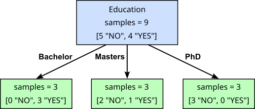
The ID3 algorithm is primarily designed for categorical data; features with (continuous) numerical features need to be discretized (e.g., converting the dollar values of Annual_Income to "low", "mid", and "high"). ID3 splits nodes by creating a new branch and child node for each possible value for the selected features. For example, ID3 would split a node using Education into three child nodes for "Bachelor", "Masters", and "PhD"; see below:
This means that, along the path from a leaf node to the root node, each feature will only be used once for a split. For example, given the example split above, when we want to further split the leaf node for the "Masters" branch, there is no need to consider "Education" anymore — after all we know that all samples in this leaf node have the same value for "Education". Other Decision Tree Learning algorithms may use the same feature for splits along the path from a leaf to the root node.
To find the best feature to be used for splitting a leaf node, ID3 uses information gain as a criterion. It measures how well a particular attribute separates the data into distinct classes — note that we do not need to consider any additional threshold here. Information gain is based on a concept from information theory called entropy, which measures the uncertainty or randomness in a dataset. By selecting the attribute that reduces entropy the most (i.e., provides the highest information gain), the ID3 algorithm ensures that each split improves the tree's ability to make accurate predictions.
One major advantage of the ID3 learning algorithm is its simplicity and ease of implementation, which makes it an excellent introduction to decision tree algorithms. Additionally, it is computationally efficient for small to medium-sized datasets with categorical attributes, making it practical for many real-world applications. However, ID3 also has notable limitations. A key drawback is its tendency to overfit the data, especially when there are attributes with many unique values or when the tree becomes too complex. It does not inherently include mechanisms like pruning to simplify the tree and prevent overfitting. Furthermore, ID3 struggles with continuous numerical data, as it only handles categorical attributes directly. Converting numerical data into categories can result in a loss of information. It also does not account for missing values in the dataset, which can lead to inaccuracies in model training and predictions.
C4.5/C5.0
The C4.5 (and its successor, C5.0) decision tree algorithms are advanced methods for building decision trees and are improvements over the earlier ID3 algorithm. They are primarily used for classification tasks. Unlike ID3, which uses information gain, C4.5 introduces the gain ratio to address a common issue where attributes with many unique values tend to dominate splits. The gain ratio normalizes the information gain by the "split information," ensuring that the algorithm selects attributes that are truly meaningful and not just overly specific.
C4.5 also stands out because it can handle both categorical and numerical attributes. For numerical data, it finds the best threshold to split the data, which makes it more versatile than ID3. Additionally, C4.5 can handle datasets with missing values by estimating the most probable values based on the existing data. This feature makes it more robust when working with real-world data, where missing values are common. Another significant improvement in C4.5 is its ability to prune the tree after it is built to address overfitting issues. The later version, C5.0, further improves on C4.5 by being faster, more memory-efficient, and better at handling large datasets.
However, there are some limitations to these algorithms. C4.5 can be computationally intensive for very large datasets, especially when dealing with numerous features or attributes. While C5.0 addresses some of these efficiency issues, the complexity of tuning hyperparameters (e.g., pruning thresholds or boosting settings) can still be a challenge. Additionally, decision trees built with these algorithms are sensitive to noisy data, as even small variations can lead to different splits, which may affect the model’s stability.
CART (Classification & Regression Trees)
The CART learning algorithm is used for both classification tasks (where the goal is to predict categories) and regression tasks (where the goal is to predict numerical values). Unlike ID3, it builds binary trees, meaning every split in the tree divides the data into exactly two parts. Most implementations of CART, including the one provided by the popular scitkit-learn library also assume that all features are numerical, potentially requiring the encoding/continuization of categorical features.
For classification problems, CART typically uses a metric called Gini impurity to choose the best attribute to split the data. Gini impurity measures how "mixed" the data is in terms of different classes; the goal is to reduce this impurity as much as possible with each split. For regression problems, CART uses the mean squared error (MSE) to determine splits, focusing on minimizing the difference between predicted and actual values.
Beyond its versatility to be used for classification and regression tasks, the CART algorithms also built-in mechanisms to support pruning to tackle overfitting, as well as handling missing values. However, CART also has limitations. Binary splits can sometimes lead to deeper trees compared to algorithms that allow multi-way splits, potentially increasing computational cost and complexity. While CART is less prone to overfitting than some other algorithms due to pruning, it still requires careful tuning of parameters like tree depth and minimum samples per split. Additionally, CART may struggle with very imbalanced datasets, where one class dominates, as it does not inherently include methods to handle such cases.
CHAID (Chi-Square Automatic Interaction Detection)
The CHAID Decision Tree learning algorithm is a statistical technique used for classification and prediction. It is unique because it relies heavily on statistical tests to determine how to split data at each step, rather than using measures like information gain or Gini impurity, as other decision tree algorithms do. Specifically, CHAID uses the chi-squared test (for categorical variables), the F-test (for continuous dependent variables), or the Bonferroni adjustment to find the most statistically significant splits.
One of the most distinctive features of CHAID is its ability to perform multi-way splits at each node, rather than just binary splits. This means that instead of dividing data into only two groups, CHAID can create multiple branches based on the number of significant categories in the data. For example, if an attribute has four categories and all are statistically relevant, CHAID might create four branches at a single node. This results in shallower trees that are easier to interpret compared to algorithms that create deep binary trees.
Another unique aspect of CHAID is that it handles categorical and ordinal data particularly well, making it popular in fields like marketing and social sciences. It evaluates all potential splits and merges categories with similar statistical properties, simplifying the tree while retaining meaningful distinctions in the data. Additionally, CHAID can handle missing values by treating them as a separate category or by using statistical estimates.
As a downside, CHAID assumes that the data relationships are adequately represented by the statistical tests it performs, which might not always capture complex patterns. Additionally, because CHAID heavily relies on statistical significance, it can be sensitive to small sample sizes or noisy data. These limitations mean that CHAID is most effective when used with clean, well-prepared datasets and when the goal is interpretability rather than high predictive accuracy.
Summary
A decision tree is a type of machine learning model that mimics human decision-making by representing decisions and their possible consequences in a tree-like structure. Each internal node in the tree represents a question or decision point based on an attribute, each branch represents a possible outcome of that decision, and each leaf node represents a final prediction or outcome. The basic idea is to split the dataset into smaller, more homogenous groups at each step, making it easier to classify data or make predictions.
One of the key reasons decision trees are important is their interpretability. Unlike many complex machine learning models, decision trees are easy to visualize and understand. They provide clear rules for how predictions are made, which is valuable in fields like healthcare, finance, or any domain where understanding the reasoning behind predictions is critical. This interpretability makes them especially useful for communicating results to non-technical stakeholders.
Decision trees are also versatile. They can handle both classification tasks, such as determining if an email is spam or not, and regression tasks, like predicting house prices. Additionally, they work well with both categorical and numerical data. Many advanced machine learning techniques, like random forests and gradient boosting machines, are built on the foundation of decision trees, making them a crucial concept to understand for anyone studying machine learning.
However, decision trees are not without limitations. They are prone to overfitting, where the model becomes too complex and captures noise in the training data instead of general patterns. Techniques like pruning and ensemble methods (combining multiple trees) help address this issue. Despite these challenges, decision trees remain a foundational and widely used tool in the machine learning toolbox. In short, decision trees are essential because of their simplicity, interpretability, and versatility. They serve as a starting point for understanding more complex models and play a crucial role in the development of many advanced machine learning methods.