
Disclaimer: This Jupyter Notebook contains content generated with the assistance of AI. While every effort has been made to review and validate the outputs, users should independently verify critical information before relying on it. The SELENE notebook repository is constantly evolving. We recommend downloading or pulling the latest version of this notebook from Github.
Dimensionality Reduction Techniques — An Overview
Modern datasets often contain a very large number of features, ranging from hundreds of variables in tabular datasets to millions of pixels in images or tokens in text data. While more data can provide richer information, high-dimensional datasets also introduce significant challenges. Machine learning models may become computationally expensive to train, more difficult to interpret, and increasingly prone to overfitting and noise. This phenomenon, often referred to as the "curse of dimensionality", motivates the need for dimensionality reduction techniques that simplify datasets while preserving their most important information.
Dimensionality reduction methods are generally divided into two major categories: feature selection and feature extraction. Feature selection focuses on identifying and retaining only the most relevant original features, thereby removing redundant or uninformative variables while preserving interpretability. In contrast, feature extraction transforms the original data into a new lower-dimensional representation that captures the underlying structure or variance of the dataset. Both approaches provide valuable tools for improving model efficiency, visualization, storage requirements, and predictive performance.
This notebook provides an overview of several widely used dimensionality reduction techniques from both categories. In addition to introducing the core concepts behind these methods, the notebook includes basic hands-on examples that demonstrate how they can be applied in practice using Python machine learning libraries. The examples are designed to build intuition for how different methods behave and when particular approaches may be most appropriate.
Learning about dimensionality reduction is important because it is a fundamental component of modern data analysis and machine learning workflows. Many real-world applications rely on the ability to efficiently process and understand complex, high-dimensional data. By understanding dimensionality reduction techniques, you can develop models that are faster, more robust, easier to visualize, and better able to generalize to unseen data. These methods therefore play a central role in both practical machine learning and exploratory data analysis.
Setting up the Notebook
Make Required Imports
This notebook requires the import of different Python packages but also additional Python modules that are part of the repository. If a package is missing, use your preferred package manager (e.g., conda or pip) to install it. If the code cell below runs with any errors, all required packages and modules have successfully been imported.
from src.utils.libimports.dimreduction import *
from src.utils.plotting.dimreduction import *
from src.utils.data.files import *
Download Required Data
Some code examples in this notebook use data that first need to be downloaded by running the code cell below. If this code cell throws any error, please check the configuration file config.yaml if the URL for downloading datasets is up to date and matches the one on Github. If not, simply download or pull the latest version from Github.
demo_data, _ = download_dataset("tabular/resources/dimreduction-demo-data.csv")
File 'data/datasets/tabular/resources/dimreduction-demo-data.csv' already exists (use 'overwrite=True' to overwrite it).
Preliminaries
- This notebooks shows several practical examples fro applying different dimensionality reduction techniques. The scope of this notebook is not a deeper introduction of individual techniques but to get the general ideas across.
Motivation
Working with High-Dimensional Data
Many real-world datasets used in data analysis, data mining, and machine learning are high-dimensional, meaning that each data instance is described by a large number of features or variables. Modern applications routinely generate enormous amounts of information from diverse sources such as sensors, social media, medical imaging, genomics, financial markets, and online platforms. For example, an image may contain thousands or millions of pixel values, a text document may be represented by tens of thousands of word frequencies, and genomic datasets may contain measurements for thousands of genes simultaneously. As data collection technologies improve, the number of recorded features continues to grow rapidly. While additional features may capture richer information about the underlying problem, they also pose significant challenges.
Computational Complexity
One of the most immediate consequences of high-dimensional data is increased computational complexity, since the runtime and memory requirements of many to most algorithms in data analysis, data mining, and machine learning depend directly on the number of features. Operations such as distance computations, matrix multiplications, covariance estimation, optimization, and model training become significantly more expensive as dimensionality grows. For example, clustering algorithms, nearest-neighbor methods, and many classification models require repeated computations across all features, causing training and inference times to increase substantially in high-dimensional spaces. As datasets continue to grow in both size and dimensionality, reducing the number of features becomes important not only for improving model quality, but also for making data processing computationally feasible.
To provide some concrete examples, the table below shows the training and, if applicable, prediction complexity of popular machine learning and data mining algorithms using the using the Big-O. In this table, $n$ denotes the number of data samples, and $d$ denotes the number of features of each sample. If the Big-O notations for the runtime complexities include additional parameters, they are defined in the "Notes" column.
| Algorithm | Training Complexity | Prediction Complexity | Notes |
|---|---|---|---|
| k-Nearest Neighbors (kNN) | $O(1)$ | $O(nd)$ | No real training but all data needs to be stored; prediction expensive in high $d$ |
| Linear Regression (OLS) | $O(nd^2 + d^3)$ | $O(d)$ | Solving normal equations; linear with gradient descent (GD) |
| Logistic Regression (GD) | $O(ndT)$ | $O(d)$ | T = number of iterations |
| Naïve Bayes | $O(nd)$ | $O(d)$ | Training involves counting; very fast |
| Decision Tree | $O(nd\log{n})$ | $O(depth) \approx O(\log{n})$ | Depends on number of splits and $depth$ of tree |
| Random Forest | $O(n_{trees}nd\log{n})$ | $O(n_{trees}\log{n})$ | $n_{trees}$ = number of trees |
| Support Vector Machine (SVM, linear) | $O(ndT)$ | $O(d)$ | $T$ = number of iterations |
| SVM (non-linear, kernel) | $O(n^2d + n^3)$ | $O(n_{supvecs}d)$ | $n_{supvecs}$ = number of support vectors |
| k-Means Clustering | $O(ndkT)$ | $O(kd)$ | $k$ = clusters, $T$ = iterations |
| DBSCAN Clustering | $O(n^2d)$ | $O(nd)$ | Assuming naive search scanning all points |
| Neural Networks (MLP) | $O(ndhT)$ | $O(dh)$ | $h$ = hidden units, $T$ = epochs |
| Gradient Boosted Trees | $O(n_{trees}nd\log{n})$ | $O(n_{trees}\log{n})$ | $n_{trees}$ = number of trees |
| Apriori (Frequent Itemsets) | Exponential in $d$ (worst case) | — | Very costly for high dimensions |
Arguably unsurprisingly, all the overall runtime of all algorithms depend on the number of features $d$, typically linearly. There is therefore a strong incentive in practice to reduce the number of features to speed up the algorithms, particularly when also the number of data samples $n$ is very or even extremely large.
Curse of Dimensionality
While the increased computational complexity relates to the efficiency of algorithms, high-dimensional datasets also pose challenges with respect to the effectiveness of algorithms (e.g., in terms of their analysis results or the quality of their predictions). The phenomena commonly observed when working with many features are collectively referred to a Curse of Dimensionality. We cover the Curse of Dimensionality in detail in a separate notebook, so here is just a brief summary of the main phenomena:
Data sparsity: Most data mining and machine learning algorithms rely on the existence of statistical patterns in the data, such as similarities, correlations, clusters, or regularities that can be learned from observed samples. However, in high-dimensional spaces, data becomes increasingly sparse because the volume of the feature space grows exponentially with the number of dimensions. As a result, even large datasets may contain too few samples relative to the size of the space, making reliable statistical estimation difficult. This sparsity often prevents algorithms from identifying statistically significant patterns and can severely degrade the performance of learning and data analysis methods.
Distance concentration: In high-dimensional spaces, the relative differences between distances tend to diminish, a phenomenon known as distance concentration. As the number of dimensions increases, most points become almost equally far away from one another, meaning that the distance to the nearest neighbor becomes nearly identical to the distance to the farthest neighbor — we visualize this phenomenon on the separate "Curse of Dimensionality" notebook. Consequently, distance measures lose their discriminative power and no longer provide meaningful information about similarity or neighborhood structure. This creates serious challenges for algorithms that rely on distances, such as k-nearest neighbors, clustering methods like k-means, and similarity search techniques, because these methods assume that nearby points are significantly more similar than distant ones. When this assumption breaks down, the quality and reliability of the resulting models and analyses can deteriorate substantially.
Overfitting and poor generalization: High-dimensional data also increases the risk of overfitting and poor generalization in machine learning models. When the number of features is very large relative to the number of available samples, models gain enough flexibility to fit not only the underlying structure of the data, but also random fluctuations and noise present in the training set. As a result, the model may achieve excellent performance on the training data while failing to generalize well to unseen data. In extreme cases, a model can memorize the training samples rather than learning meaningful patterns. This problem becomes particularly severe in high-dimensional spaces because the abundance of features increases the likelihood of finding spurious correlations that do not reflect true relationships in the underlying data-generating process.
In principle, many of the problems associated with the Curse of Dimensionality could be mitigated by collecting more data samples. Since high-dimensional spaces are extremely sparse, increasing the number of observations can improve data density, making statistical estimation more reliable and helping machine learning algorithms identify meaningful patterns. With sufficient data, distances between points become more informative, overfitting can be reduced, and models are more likely to generalize well to unseen samples. From this perspective, the Curse of Dimensionality is not an inherent impossibility, but rather a consequence of having insufficient data relative to the dimensionality of the feature space.
However, the major challenge is that the amount of data required grows exponentially with the number of dimensions. As each additional feature expands the size of the feature space, vastly more samples are needed to maintain the same coverage or density of observations. In practice, this quickly becomes computationally, financially, and physically infeasible. Collecting, storing, and processing exponentially increasing amounts of data is often impossible in real-world applications.
Overall Goal
Given the challenges we have just discussed, a common goal is to reduce the number of features in high-dimensional datasets to improve both the efficiency and effectiveness of data analysis/mining and machine learning algorithms. Although reducing the number of features appears to be a natural solution, determining which features can safely be removed is far from trivial. In many real-world datasets, it is difficult to assess a priori which variables contain important information and which are irrelevant or redundant. A feature that appears uninformative when considered in isolation may still become highly valuable when combined with other features. Consequently, simply removing variables based on individual statistics or intuition can lead to the loss of important information and degrade the performance of subsequent data analysis or machine learning tasks.
This task becomes even more pronounced when interactions between multiple features influence the underlying patterns in the data. Many machine learning models rely not only on the individual predictive power of features, but also on complex dependencies and relationships among them. For example, two features may each appear weakly informative on their own, yet together provide strong predictive capability. As a result, dimensionality reduction requires carefully balancing the removal of redundancy and noise against the risk of discarding meaningful structure hidden within feature interactions. Let's therefore have a look at the basic strategies for dimensionality reduction next.
Basic Strategies
In general, there are two fundamental strategies for reducing the dimensionality of a dataset: feature selection and feature reduction. Feature selection aims to identify and retain only a subset of the original features that are considered most relevant, while discarding irrelevant or redundant variables. In contrast, feature extraction transforms the original features into a new set of lower-dimensional variables that attempt to preserve the most important information contained in the data. Both approaches seek to mitigate the challenges associated with high-dimensional data, such as computational complexity, overfitting, and sparsity, while improving the efficiency and effectiveness of subsequent data analysis and machine learning tasks.
Feature Selection
Feature selection is arguably the most intuitive approach to dimensionality reduction because it directly attempts to reduce the number of variables by removing features from the dataset. In many cases, there are straightforward reasons for eliminating a feature, such as missing values, constant attributes, duplicated information, or variables that are clearly irrelevant to the analysis task. However, other decisions are far less obvious. Some features may appear unimportant when considered individually, yet still contribute valuable information through interactions with other variables. Consequently, effective feature selection requires carefully distinguishing between truly irrelevant features and those that participate in meaningful underlying patterns within the data.
Manual Assessment
The most common approach to remove individual features is to "manually" identify features (i.e., without any kind of analysis) that should not be considered for any analysis or model learning based on best practices or domain knowledge. To give some examples, consider the table below that shows a dataset of bank customers to train a classification model to decide whether a customer is likely to default on their credit. The dataset has no expectation to be realistic; also assume that this is the complete dataset.
| ID | DOB | Ethnicity | Verified | Marital Status | Annual Income | Acc. Balance | Acc. Open Date | Credit Default | |
|---|---|---|---|---|---|---|---|---|---|
| C001 | alice@... | 1988-03-12 | Hispanic | Yes | N/A | 85000 | 12500 | 2016-05-10 | No |
| C002 | brian@... | 1995-07-21 | Asian | Yes | Single | 54000 | 3200 | 2020-08-15 | No |
| C003 | charles@... | 1979-11-02 | White | Yes | N/A | 120000 | 45200 | 2012-01-20 | No |
| C004 | diana@... | 1992-01-18 | Hispanic | Yes | N/A | 47000 | -850 | 2021-11-05 | Yes |
| C005 | ethan@... | 1985-09-30 | Black | Yes | N/A | 76000 | 9800 | 2017-04-28 | No |
| C006 | fiona@... | 1998-06-14 | Asian | Yes | N/A | 39000 | 1100 | 2023-02-11 | No |
| C007 | george@... | 1975-12-25 | Black | Yes | Married | 150000 | 87500 | 2010-09-03 | No |
| C008 | hannah@... | 1990-04-09 | Black | Yes | N/A | 68000 | 5400 | 2018-07-19 | No |
| C009 | ivan@... | 1983-08-27 | White | Yes | Widowed | 59000 | -2300 | 2015-12-01 | Yes |
| C010 | jasmine@... | 1996-10-05 | Hispanic | Yes | N/A | 44000 | 2600 | 2022-06-22 | No |
Assuming that the column "Credit Default" represents the target of our classification task, all remaining columns are potential features used to train a classifier. However, just by inspecting the data, the are arguably a few columns we should not consider features and therefore remove before the training:
ID: Unique identifiers are typically removed from datasets because they generally do not carry any semantic meaning relevant to the underlying analysis or prediction task. Their primary purpose is merely to distinguish individual records, not to describe meaningful properties of the data instances themselves. Since IDs are usually arbitrary values, machine learning models cannot derive useful patterns from them. In some cases, retaining unique identifiers may even be harmful, as models could incorrectly memorize specific records rather than learning generalizable relationships.
Email: Similar to IDS, email addresses primarily serve as unique identifiers for individuals rather than describing behavioral, demographic, or statistical properties that a machine learning model can meaningfully generalize from. Additionally, email addresses constitute personally identifiable information (PII), raising important privacy and data protection concerns. Consequently, removing email addresses is both a common feature selection step and an important measure for preserving user privacy and ensuring compliance with data protection regulations.
Ethnicity: Removing attributes such as ethnicity is often recommended in order to reduce the risk of biased or discriminatory decision-making. Machine learning models trained on sensitive demographic information may unintentionally learn and reinforce historical or societal biases, potentially leading to unfair outcomes in applications such as credit approval, loan pricing, or risk assessment. Furthermore, in many jurisdictions, making financial decisions based on protected attributes such as ethnicity may violate anti-discrimination laws and ethical guidelines.
Verified: Assuming that the table shows all customers, the value for "Verified" is the same for all customers. Features that have the same value for all samples can typically be removed because they do not provide any discriminative or informative content. Since the feature never changes across the dataset, it cannot help distinguish between different data instances or contribute to identifying meaningful patterns, correlations, or predictive relationships. From a statistical perspective, such features have zero variance and therefore contain no usable information for most data analysis or machine learning algorithms. Retaining them only increases dimensionality and computational overhead without improving model performance.
Marital Status: Again, assuming that the table shows all customers, we see that for most of the customers, we do not know their marital status. Features containing a large proportion of missing values are often removed because they may provide too little reliable information for meaningful analysis or model training. When most entries of a feature are absent, it becomes difficult to estimate its true statistical behavior or relationships with other variables. Although missing values can sometimes be imputed, heavy imputation may introduce noise, bias, or artificial patterns into the dataset. Furthermore, retaining highly incomplete features increases data complexity while often contributing little predictive value.
Although seemingly straightforward, manually assessing whether features should be removed is often not obvious in practice, since the usefulness of a feature strongly depends on the specific dataset, application domain, and learning task. A feature that appears irrelevant in one context may become highly informative in another, particularly when complex interactions with other variables exist. Furthermore, the importance of a feature may vary depending on the chosen machine learning model and the objective of the analysis. Just to give some counterexamples for our features above:
- Some IDs do carry some information, for example, if an ID is derived from a time stamp (e.g., when the bank customer signed on)
- There are studies that aim to predict a person's personality traits from their choice of email addresses; while a bit of a long shot, these personality traits could be used as features.
- If the whole purpose of a task is to actually identify biases (e.g., "Does ethnicity affect the income?"), we obviously can remove the relevant features.
Data-Driven Assessment
Data-driven assessment for feature selection typically involves much more than simply “looking” at the data to decide which features to remove. Instead, it relies on quantitative techniques and statistical evidence to evaluate how useful, redundant, or noisy each feature is with respect to the predictive task. Such quantitative techniques can be further categorized into filter methods, wrapper methods, and embedded methods.
To provide some basic examples for each method, we consider a very simple demo dataset for a regression task. The dataset contains $100$ samples, and $5$ numerical features $x_1$, $x_2$, ..., $x_5$ and a numerical target variable $y$; the data does not capture any real-world phenomenon. Let's load the dataset from the file into Pandas DataFrame and have a quick look at the data.
df = pd.read_csv(demo_data)

df.head()
| x1 | x2 | x3 | x4 | x5 | y | |
|---|---|---|---|---|---|---|
| 0 | 0.496714 | -0.173585 | 0.299358 | -1.276229 | 0.541989 | 0.702740 |
| 1 | -0.138264 | -0.766306 | 0.299561 | -1.261162 | 0.355263 | -1.893866 |
| 2 | 0.647689 | 1.276507 | 0.300083 | -0.606520 | 3.442609 | 13.734696 |
| 3 | 1.523030 | 3.005297 | 0.300054 | -0.706882 | 5.112901 | 23.920814 |
| 4 | -0.234153 | -0.746669 | 0.297622 | 1.701185 | -3.502008 | -11.390148 |
We also convert the DataFrame into NumPy arrays X and y to represent the data as a feature matrix and target vector, respectively.
X = df.iloc[:,0:-1].to_numpy()
y = df.iloc[:, -1].to_numpy()
Filter Methods
The basic idea behind filter methods for feature selection is to evaluate the usefulness of features using statistical properties of the data, independently of any specific machine learning model. Each feature is assessed according to some criterion that measures its relevance, informativeness, or redundancy, and features that appear uninformative are removed before model training. Typical evaluation criteria include variance, correlation, mutual information, chi-square statistics, or measures of dependency with the target variable. Because filter methods do not require repeatedly training predictive models, they are usually computationally efficient and scalable to high-dimensional datasets.
A key characteristic of filter methods is that they treat feature selection as a preprocessing step that is separate from the learning algorithm itself. This makes them simple, fast, and broadly applicable across different machine learning models. However, since features are often evaluated individually, filter methods may fail to capture complex interactions or dependencies between multiple variables. Consequently, while filter methods are useful for quickly removing obviously irrelevant or redundant features, they do not always identify the optimal feature subset for a specific predictive task.
A simple and commonly used filter method for feature selection is to remove features with very low variance across the dataset. The motivation behind this approach is that features that barely change from one observation to another contain little information that can help distinguish between different samples or predict the target variable — note that we already covered the obvious case where all samples have exactly the same value for a feature. For example, a feature that has nearly the same value for almost all data points contributes little to identifying patterns or relationships in the data.
Let's check the variances for our $5$ features of our demo dataset. Pandas provides the very useful method var() to compute the variance for all numerical features in a DataFrame:
df.var()
x1      0.824770
x2      5.473525
x3      0.000001
x4      2.619240
x5     11.903910
y     222.106821
dtype: float64
As the results show, the values for feature $x_3$ have a very low variance, meaning that most values for this feature are almost the same; and you can see this by just looking at the few raw samples shown above. This makes $x_3$ and potential candidate feature to be removed, as it unlikely to capture any useful relationships or patterns that would help with the regression task
Important: There are practical situations where low-variance features can still be useful and should not be removed as part of feature selection. A feature may vary only slightly overall but still contain important information for distinguishing rare but critical cases, such as fraud detection, medical diagnosis, or anomaly detection. For example, a biomarker that is nearly constant for most patients but changes subtly for individuals with a disease may have low variance yet strong predictive power. Therefore, variance-based filtering is only a simple heuristic and should ideally be combined with methods that evaluate the actual relationship between features and the prediction target — and generally require a good understanding of the data and the task.
Again, Pandas provides and convenient method corr() to compute all pairwise correlation (by default: Pearson Correlation Coefficient) between numerical columns in a DataFrame. The result of this method is itself a DataFrame representing the correlation matrix containing all pairwise correlations. The code cell below applies the method on our demo dataset using the Pearson Correlation Coefficient, meaning that all values are between $-1.0$ (perfect negative correlation) and $+1.0$ (perfect positive correlation), and with $0.0$ indicating no correlation at all.
correlation_matrix = df.corr()

correlation_matrix
| x1 | x2 | x3 | x4 | x5 | y | |
|---|---|---|---|---|---|---|
| x1 | 1.000000 | 0.914840 | 0.190840 | -0.252812 | 0.740295 | 0.884503 |
| x2 | 0.914840 | 1.000000 | 0.170268 | -0.236759 | 0.785111 | 0.925800 |
| x3 | 0.190840 | 0.170268 | 1.000000 | -0.837603 | 0.743990 | 0.517800 |
| x4 | -0.252812 | -0.236759 | -0.837603 | 1.000000 | -0.687005 | -0.486640 |
| x5 | 0.740295 | 0.785111 | 0.743990 | -0.687005 | 1.000000 | 0.953232 |
| y | 0.884503 | 0.925800 | 0.517800 | -0.486640 | 0.953232 | 1.000000 |
To better visualize the correlation matrix, we provide the auxiliary method plot_correlation_matrix(); just run the code cell below.
plot_correlation_matrix(correlation_matrix)

With respect to a regression task — as our demo dataset represents — there are two cases that are relevant in the context for feature selection:
Low correlation between feature and target: A low correlation between a feature and the target variable may indicate that the feature has little predictive value and could potentially be removed during feature selection. If changes in the feature are not associated with meaningful changes in the target, the feature is less likely to help the model learn useful patterns.
High correlation between two features: A high correlation between two features (e.g., between $x_1$ and $x_2$) can cause problems because both features may contain largely redundant information. This redundancy can increase model complexity without adding meaningful predictive power and may lead to issues such as multicollinearity, where the model struggles to determine the individual effect of each feature. In some models, especially linear models, this can result in unstable parameter estimates and reduced interpretability. Therefore, when two features are highly correlated, it is often beneficial to remove one of them to simplify the model and reduce redundancy.
Important: Feature selection based solely on pairwise linear correlation must be applied with great care because important relationships in the data may not be captured by simple two-feature comparisons. In some cases, a feature may appear only weakly related to the target or to another feature when considered individually, but it may become highly informative when combined with several other features. Such higher-order interactions cannot be detected through pairwise correlation analysis alone, meaning that useful features could be removed incorrectly. In addition, standard correlation measures such as Pearson correlation only capture linear relationships. Two variables may have a strong nonlinear dependency while still exhibiting a very low linear correlation coefficient. For example, a quadratic or circular relationship between variables may not be recognized by linear correlation analysis even though the variables are clearly related. As a result, relying only on pairwise linear correlation can overlook important nonlinear patterns and lead to poor feature selection decisions.
Wrapper Methods
The basic idea behind wrapper methods for feature selection is to evaluate subsets of features by directly measuring how well a machine learning model performs when trained on those features. Instead of relying solely on statistical properties of the data, wrapper methods repeatedly train and evaluate a predictive model using different feature combinations. The quality of a feature subset is therefore determined by the resulting model performance, such as classification accuracy or prediction error. In this sense, the feature selection process “wraps around” the learning algorithm itself.
Wrapper methods typically employ a search strategy to explore possible feature subsets, for example by iteratively adding, removing, or ranking features. Common approaches include forward selection, backward elimination, and recursive feature elimination. Because wrapper methods evaluate features in the context of the actual model, they can capture complex interactions and dependencies between variables that simpler filter methods may overlook. However, this increased flexibility comes at the cost of significantly higher computational complexity, since many models may need to be trained and evaluated during the search process.
To see an example, let's apply RFECV (Recursive Feature Elimination with Cross-Validation) on our example dataset. RFCEV automatically determines an optimal subset of features by repeatedly training a model, removing the least important features, and evaluating model performance using cross-validation. The process begins with all features, trains the chosen estimator, ranks features according to their importance, removes the weakest features, and repeats this procedure recursively until only a small number of features remain. At each stage, cross-validation is used to estimate predictive performance, allowing RFECV to identify the feature subset that achieves the best balance between model complexity and predictive accuracy.
RFECV is directly supported by the scikit-learn library, making it very simple to perform feature selection. The code below creates a RandomForestRegressor with 200 Decision Trees and uses it together with RFECV. The latter repeatedly trains the random forest model, ranks features according to their importance, removes the least important feature at each iteration (step=1), and evaluates predictive performance using 5-fold cross-validation (KFold). The scoring metric "neg_mean_squared_error" is used to assess regression quality, where lower prediction error corresponds to better performance.
rf_model = RandomForestRegressor(n_estimators=200)

selector = RFECV(
    estimator=rf_model,
    step=1,
    cv=KFold(5, shuffle=True, random_state=42),
    scoring="neg_mean_squared_error",
    n_jobs=-1
).fit(X, y)
You will notice that executing the previous code cell is likely to take a few seconds; after all, we are training $200$ Decision Trees and performing 5-fold cross-validation. However, our dataset contains only $100$ data samples and $5$ features. So you can imagine how RFECV will perform on large datasets with many more features!
In any case, we can now the names of the features selected by the fitted RFECV object and convert them into a NumPy array for convenient display. The expression df.columns[0:-1] selects all column names except the last one, which is our target variable. The boolean mask selector.support_ indicates which features were retained by RFECV, and applying this mask filters the column names accordingly. Finally, .to_numpy() converts the selected feature names into a NumPy array.
selected_features = df.columns[0:-1][selector.support_].to_numpy()

print(f"Selected features: {selected_features}")
Selected features: ['x1' 'x2' 'x5']
Beyond just the selected features, can also create a ranked table of feature importance based on the results produced by RFECV. The array selector.ranking_ contains the rank assigned to each feature. A Pandas Series is constructed using the feature names from df.columns[0:-1] as the index, allowing each rank to be associated with its corresponding feature. The features are then sorted by rank using .sort_values(), converted into a DataFrame with .to_frame(), and the default column name is renamed to "Rank". Finally, ranking.head() displays the top-ranked features in the resulting table.
ranking = pd.Series(selector.ranking_, index=df.columns[0:-1]).sort_values().to_frame().rename(columns= {0: 'Rank'})

ranking.head()
| Rank | |
|---|---|
| x1 | 1 |
| x2 | 1 |
| x5 | 1 |
| x4 | 2 |
| x3 | 3 |
When using RFECV, multiple features having the same top rank typically means that the algorithm considers all of those features equally important in the final selected subset. In sklearn, features assigned rank 1 are the features retained after the recursive elimination process has determined the optimal number of features according to the chosen scoring metric and cross-validation performance. This does not necessarily imply that all rank-1 features contribute equally or independently to the model, but rather that they survived the elimination process together. In many cases, several highly informative or correlated features may all receive the top rank because removing any one of them would not sufficiently improve model performance to justify elimination.
Beyond RFECV, there are several other commonly used wrapper methods for feature selection. These methods differ mainly in how they search through possible feature subsets.
One of the simplest approaches is forward selection, where the algorithm starts with no features and iteratively adds the feature that most improves model performance. The opposite strategy is backward elimination, which begins with all features and repeatedly removes the least useful feature until performance deteriorates or a desired number of features remains. A related method is Recursive Feature Elimination (RFE), which recursively removes the least important features according to a trained estimator, but unlike RFECV, it does not automatically determine the optimal number of features through cross-validation.
More advanced wrapper approaches include heuristic and stochastic search methods such as genetic algorithms, simulated annealing, and sequential floating selection. These methods attempt to explore the space of possible feature subsets more flexibly than simple greedy procedures. For example, sequential floating selection can both add and remove features dynamically during the search process, helping to avoid poor local decisions made by purely forward or backward strategies. While these approaches can sometimes identify better feature subsets, they are generally more computationally expensive because they require repeatedly training and evaluating predictive models on many different feature combinations.
Embedded Methods
The basic idea behind embedded methods for feature selection is to perform feature selection automatically as part of the model training process itself. In contrast to filter methods, which evaluate features independently of a learning algorithm, and wrapper methods, which repeatedly train models on different feature subsets, embedded methods integrate feature selection directly into the construction of the predictive model. As the model learns from the data, it simultaneously determines which features are most important for the prediction task.
Many embedded methods achieve this by assigning importance scores or penalties to features during optimization. For example, decision trees and random forests estimate feature importance based on how much a feature improves the quality of splits. For an example, let's actually train a Random Forest regressor with $200$ Decision Trees on our example dataset.
forest = RandomForestRegressor(n_estimators=200, random_state=0).fit(X, y)
We can now compute feature importance statistics from a trained Random Forest model. The expression forest.feature_importances_ returns the overall importance score of each feature, typically based on the average reduction in impurity contributed by that feature across all trees in the forest. The second line calculates the standard deviation of these importance scores across the individual decision trees contained in forest.estimators_. This provides a measure of how consistent the estimated importance of each feature is throughout the ensemble. Features with large standard deviations may have importance values that vary substantially between trees, while small standard deviations indicate more stable and consistent feature importance estimates.
importances = forest.feature_importances_

std_devs = np.std([tree.feature_importances_ for tree in forest.estimators_], axis=0)
To inspect the results the code cell generates a bar plot with error bars where the height of the bars indicate the feature importance score for all $5$ features and the error bars represent the standard deviation for each feature.
feature_names = [f"x{i+1}" for i in range(X.shape[1])]

plot_feature_importances(importances, std_devs, feature_names)

According to this plot features $x_5$ and $x_2$ are the most important ones, followed by $x_1$. The scores for $x_3$ and $x_4$ are very low, indicating that these two features can probably be removed with hurting the accuracy of the model.
Most machine learning models provide some well-defined mechanism for quantifying the importance or influence of individual features based on their internal learning process. The exact notion of feature importance depends on the underlying model architecture and optimization procedure. For example, linear models often measure importance through the magnitude of learned coefficients, while Decision Trees and ensemble methods evaluate how much a feature contributes to reducing impurity or improving prediction quality during splitting (cf. example above). Similarly, regularized models may suppress irrelevant features by shrinking their parameters toward zero. These internally derived importance measures make it possible to perform feature selection directly as part of the model training process, which forms the basis of embedded feature selection methods.
In general, since embedded methods perform feature selection directly during model optimization, they avoid the expensive repeated retraining procedures required by many wrapper methods. As a result, they are often significantly more computationally efficient, especially for high-dimensional datasets. At the same time, because the learning algorithm evaluates features in the context of the full model, embedded methods can capture important interactions, nonlinear relationships, and dependencies between variables that simpler filter methods may overlook. However, an important limitation is that the resulting feature importance estimates are inherently model-dependent. Different learning algorithms may assess feature relevance according to very different criteria, meaning that a feature considered highly important by one model may appear far less relevant to another. Consequently, the selected feature subset is often closely tied to the assumptions, structure, and optimization behavior of the specific model used during training.
Feature Extraction
Feature extraction aims to reduce the number of features by transforming the original set of features into a new set of derived features. Instead of simply removing existing features, feature extraction combines or transforms information from the original variables in such a way that the new features still capture the most important characteristics of the data. In many cases, the number of newly generated features can be significantly smaller than the number of original features, which helps reduce dimensionality, computational cost, and the risk of overfitting. Different feature extraction methods vary in how these new features are constructed from the original data, and can be categorized into linear methods, manifold learning methods, and neural network methods.
Linear Methods
The basic idea behind linear methods for feature extraction is to create new features as linear combinations of the original features. These methods transform the data into a new feature space where the most important information is concentrated in a smaller number of derived variables. Typically, the transformation is designed to preserve certain properties of the data, such as maximizing variance, preserving distances, or improving class separability. Popular linear methods include:
- Principal Component Analysis (PCA)
- Linear Discriminant Analysis (LDA)
- Independent Component Analysis (ICA)
- Singular Value Decomposition (SVD)
- Canonical Correlation Analysis (CCA)
Side note: Many of these methods provide extensions or variants for nonlinear dimensionality reduction. However, we refer to the basic linear approaches.
Fundamentally, all linear methods for feature extraction aim to determine some form of transformation matrix that maps the original feature space into a new feature space. The rows or columns of this matrix define how the original features are combined to form the new features. The original feature space is typically our original feature matrix $\mathbf{X}\in \mathbb{R}^{n\times d}$, where $n$ is the number of data samples, and $d$ is the number of features. We know want to transform or project $\mathbf{X}$ into lower-dimensional space represented by a new feature matrix $\mathbf{P}\in\mathbb{R}^{n\times p}$, where $p$ is then number of new features in the projected space. Naturally, we want $p < n$ or typically even $p \ll n$. To this end, we need to a transformation matrix $\mathbf{W}\in\mathbb{R}^{d\times p}$ such that:
In principle, any transformation matrix $\mathbf{W}$ with suitable dimensions can map the original feature matrix into a lower-dimensional space. However, most arbitrary transformations would discard important structure or information contained in the data. The overall goal of linear feature extraction is therefore to identify a transformation matrix that reduces dimensionality while preserving as much relevant information as possible. And this is where different approaches for linear methods can be distinguished from each other — that is, by their use of different criteria to determine the "best" transformation matrix $\mathbf{W}$.
For a concrete example, let's consider Principal Component Analysis (PCA). PCA directly addresses the observation that reducing the dimensionality of a datasets results in datasets to be more dense — something we actually want! However, if the transformation is chosen poorly, many points may become "clumped together" making the reduced representation less informative and potentially harming subsequent analysis or learning tasks. As such, PCA for a projection where data exhibits the largest possible spread, measured by variance. By maximizing the variance of the projected data, PCA attempts to preserve the most important structure of the data even after dimensionality reduction, thereby minimizing the loss of information.
To illustrate the basic idea behind PCA, consider the three plots below; all three plots show the same original $2$-dimensional dataset (blue points). The goal is to reduce the number dimensions of this dataset from $2$ to just $1$. One naive transformation would be to simply ignore the feature $x_1$ which is analogous to mapping all data points to the $x_2$-axis (left plot). Notice how the data (red points) is now bunched together, thus potentially losing useful patterns and information. Alternatively, we could map the data onto the $x_1$-axis by ignoring the feature $x_2$ (middle plot). This transformation is arguably a bit better since the projected data is more spread out. However, the right plot shows the result of PCA which transforms the data in such a way that the spread, measured by the variance of the projected data is maximized.
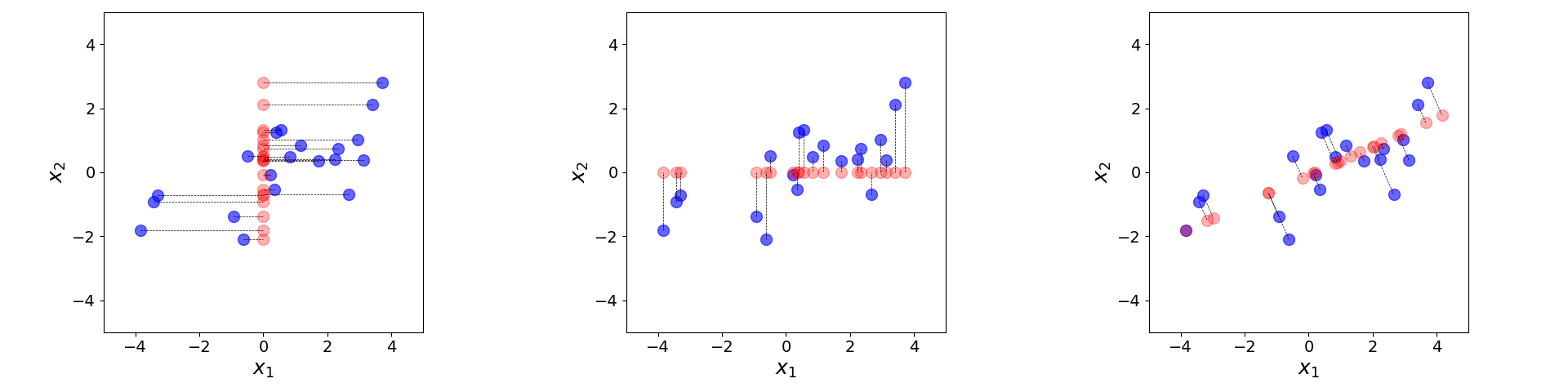
Side note: The red data points in the right plot still seem to have an $x_1$ and $x_2$ value. This is because the plots where the projected data points would lie in the original $2$-dimensional space. The real output of PCA for this example is a $1$-dimensional dataset with a feature, say, $x^\prime$ which is a linear combination of $x_1$ and $x_2$.
For a practical example, we can apply PCA on our demo dataset containing $5$ features. The scikit-learn library includes a built-in implementation of PCA that makes dimensionality reduction straightforward and efficient. With only a few lines of code, you can fit a PCA model, choose the number of principal components, and transform high-dimensional data into a lower-dimensional representation. The code cell below uses this implementation to reduce the number of dimensions of our demo dataset from $5$ down to $2$.
X_pca = PCA(n_components=2).fit_transform(X)
Now that we have a $2$-dimensional dataset, we can easily plot it using the provided auxiliary method plot_2d_projection(). Note that we use $x^\prime$ and $x^{\prime\prime}$ to denote the two new features. But again, both features derives from some linear combinations of the original $5$ features $x_1$, $x_2$, ..., $x_5$.
plot_2d_projection(X_pca, colors="blue")

Important: Reducing a dataset to two dimensions with PCA and visualizing the result can be useful for gaining intuition about the structure of the data, such as identifying clusters or trends. However, such a visualization alone does not provide any guarantee about the quality of the transformation. A 2D projection may omit important variance present in the original high-dimensional space, potentially distorting distances, class separability, or other relevant relationships between samples. In practice, the effectiveness of PCA must therefore be evaluated using quantitative metrics. Common measures include the explained variance ratio, reconstruction error, or downstream model performance after dimensionality reduction. These metrics help determine how much information is retained or lost when reducing dimensionality and whether the transformed representation remains suitable for the intended analytical task. Such considerations go beyond the scope of this overview, however.
PCA and some other linear are unsupervised methods, meaning that they only use the feature data itself and do not take target labels or class information into account. Their goal is typically to preserve important structures in the data, such as variance or similarity relationships, without considering any specific prediction task. As a result, the extracted features may capture general patterns in the data but are not necessarily optimized for classification performance. However, there are also supervised feature extraction methods that explicitly incorporate class labels into the dimensionality reduction process. These methods aim not only to reduce dimensionality but also to improve the separation between different classes in the projected space.
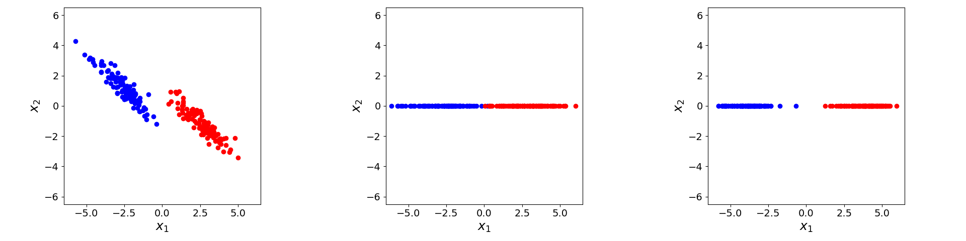
A well-known example for a supervised linear method is Linear Discriminant Analysis (LDA), which searches for transformations that maximize class separability while minimizing variation within the same class. To see the benefits of LDA over PCA for a labeled dataset, consider the $2$-dimensional dataset shown in the left plot below. Again, we want to reduce the dataset from $2$ dimensions to $1$ dimensions. If we would use PCA — which is unsupervised and therefore agnostic to the class labels — we would get the result as shown in the middle plot. In this result, data points of different classes now overlap, negatively affecting the accuracy of any trained classifier. In contrast, the right plot shows the result when using LDA. Since LDA takes the class labels into account, it is able to preserve the separation between the classes.
Linear dimensionality reduction techniques such as Principal Component Analysis (PCA) and Linear Discriminant Analysis (LDA) assume that the essential structure of the data can be represented as linear combinations of the original features. PCA assumes that the directions of maximum variance capture the most important information in the dataset, while LDA assumes that classes can be separated through linear boundaries and that class distributions are approximately Gaussian with similar covariance structures. In both cases, the methods project the data onto a lower-dimensional linear subspace while attempting to preserve either variance (PCA) or class separability (LDA).
The main limitation of these approaches is that they cannot effectively capture complex nonlinear relationships that are often present in real-world data. If the data lies on a curved manifold or exhibits intricate structures, linear projections may fail to preserve important patterns and can lead to significant information loss. Furthermore, PCA is sensitive to feature scaling and outliers, while LDA may perform poorly when its statistical assumptions are violated or when the number of features exceeds the number of samples. As a result, nonlinear dimensionality reduction techniques are often preferred for more complex datasets.
Manifold Learning
In the context of a dataset, a manifold is a lower-dimensional structure embedded within a higher-dimensional space on which the data approximately lies. Although each data point may be described using many features, the true underlying degrees of freedom governing the data can be much smaller. A popular synthetic example is the so-called Swiss roll manifold. It consists of a two-dimensional surface that has been smoothly rolled into a spiral shape within three-dimensional space, resembling a rolled sheet of paper. The figure below shows an example plot generated using the auxiliary method make_swiss_roll() of the scikit-learn library. The colors of the data points indicate their closeness or similarity in the manifold — points of similar color are more similar to each other then points with (very) different colors.
X_roll, c_roll = make_swiss_roll(n_samples=2000, random_state=0)

plot_swiss_roll(X_roll, c_roll)

Important: Although each data point is represented with $3$-dimensional coordinates, the intrinsic dimensionality of the dataset is only $2$ because every point can essentially be described by its position along the surface of the sheet. The key idea is that meaningful relationships between points are defined by distances measured along the manifold rather than through ordinary straight-line Euclidean distances in the surrounding 3D space. Two data points are therefore considered far away if they are separated by a large distance when traveling along the surface of the roll, even if they appear close in 3D space. For example, points located on adjacent layers of the rolled sheet may have a small Euclidean distance because the layers physically lie near each other, but they are actually distant on the manifold since moving from one point to the other would require traversing a long path along the rolled surface. Notice how some points with very different colors are close together with respect to their Euclidean coordinates.
Let's see what happens if we use a linear method such as PCA to reduce the dimensionality of the $3$-dimensional Swiss roll down to $2$ dimensions. The plot below shows the output after using the PCA implementation of scikit-learn as done before.
X_roll_pca = PCA(n_components=2).fit_transform(X_roll)

plot_2d_projection(X_roll_pca, colors=c_roll)

At a first glance, you might think that PCA is doing a good job since it preserves the "spiral" of the Swiss roll. However, keep in mind that distances between the data points in the Euclidian space do reflect the similarity/closeness of the points in the manifold. The example region highlighted in the plot above shows points that are far away along the mainfold — notice the very different colors — but are seemingly close in the $2$-dimensional Euclidean space. Any linear dimensionality reduction method would yield a similar result.
Manifold learning methods fundamentally differ because they are built around the idea of preserving locality. These methods construct local neighborhoods of nearby points and attempt to maintain these neighborhood relationships in the lower-dimensional embedding. Instead of modeling the data globally as a flat subspace, they assume the data lies on a nonlinear manifold that can locally be approximated as linear. By preserving local distances or neighborhood connectivity, manifold learning methods can "unfold" complex nonlinear structures that linear techniques cannot represent, making them especially powerful for visualizing and analyzing high-dimensional data with nonlinear geometry. Some popular manifold learning methods include:
- t-Distributed Stochastic Neighbor Embedding (t-SNE)
- Uniform Manifold Approximation and Projection (UMAP)
- Locally Linear Embedding (LLE)
- Laplacian Eigenmaps
- Isomap
As mentioned earlier, there are also extensions to linear methods to support nonlinear mappings. For example Kernel PCA extends linear PCA using nonlinear kernel functions to meaningfully reduce the dimensionality of manifolds.
For a concrete example, let's consider t-Distributed Stochastic Neighbor Embedding (t-SNE). The basic idea behind t-SNE (t-Distributed Stochastic Neighbor Embedding) is to represent distances between data points in terms of probabilities rather than raw Euclidean distances. In the original high-dimensional space, t-SNE assigns a high joint probability to pairs of points that are close neighbors and a low probability to points that are far apart. These probabilities can be interpreted as the likelihood that two points would “pick” each other as neighbors. In the lower-dimensional embedding, t-SNE defines a second probability distribution over the projected points using a Student’s t-distribution, which helps avoid crowding points together.
Because probabilities are dimensionless, the method can directly compare the neighborhood structure of the original and projected spaces, even though they have different dimensionalities. t-SNE then optimizes the embedding such that the two probability distributions become as similar as possible, typically by minimizing the Kullback–Leibler divergence between them. As a result, nearby points in the original space remain nearby in the visualization, meaning that local neighborhoods are preserved. This makes t-SNE particularly effective for revealing clusters and local structures in complex high-dimensional datasets. Again, scikit-learn provides an implementation for t-SNE, so we can apply it to the Swiss roll manifold:
X_roll_tsne = TSNE(n_components=2, learning_rate='auto', init='random', perplexity=50).fit_transform(X_roll)
One of the most important input arguments for t-SNE is the perplexity parameter. The perplexity parameter in t-SNE controls the effective size of the local neighborhood that each data point considers when constructing the probability distribution of neighbors. Intuitively, it determines the balance between focusing on very local structure versus incorporating a broader view of the data. A small perplexity value makes t-SNE pay attention only to very close neighbors, often producing many small, tightly separated clusters. A larger perplexity considers more neighbors and therefore captures more global structure, leading to smoother and more connected embeddings.
In practice, typical values range between 5 and 50, depending on dataset size and structure. Try running the code cell above with different values for perplexity to see how it affects the result. In general, you will notice that running t-SNE is likely to take a few seconds. t-SNE is generally much more computationally expensive than PCA because it must compute and iteratively optimize pairwise similarities between many data points in both the high-dimensional and low-dimensional spaces. This involves constructing neighborhood probability distributions and repeatedly updating point positions through nonlinear optimization. In contrast, PCA mainly requires a single linear algebra operation which can be computed very efficiently. Consequently, t-SNE scales much worse with dataset size, especially for large numbers of samples.
To inspect the result, we can again plot data points in the lower-dimensional projected space.
plot_2d_projection(X_roll_tsne, colors=c_roll)

You should see that with perplexity values between $25$ and $50$ here, t-SNE is quite capable to "unroll" the manifold by preserving local neighborhoods but also pushing data points that are far away in the manifold also far away in the projects $2$-dimensional space.
Important: Nonlinear dimensionality reduction methods such as t-SNE are primarily designed to preserve local neighborhood relationships rather than global geometry. As a result, distances between clusters in a t-SNE visualization are often not meaningful: clusters that appear far apart may not actually be very different in the original space, while nearby clusters may not truly overlap. Similarly, the relative sizes, densities, and shapes of clusters can become distorted because the optimization process focuses on maintaining local similarities instead of preserving global distances or variance structure. Therefore, t-SNE is highly effective for visualization and exploratory analysis, but its embeddings should be interpreted cautiously when drawing conclusions about global structure or quantitative distances.
Neural Network Methods
Linear methods like PCA act as rigid, flat mirrors: they project data onto a straight subspace, which works beautifully if your data is just stretched out, but completely fails if the data is bent, curved, or twisted. Traditional manifold learning methods like t-SNE or UMAP solve this by acting like flexible graph paper; they bend and wrap themselves around the data's local neighborhoods to unroll complex, non-linear shapes. However, these classical manifold methods are non-parametric, meaning they only learn how to rearrange the specific data points they are given. If you get new data tomorrow, you can't easily map it without rerunning the entire optimization process from scratch, as they don't learn an underlying mathematical function.
In contrast neural network-based methods combine the non-linear flexibility of manifold learning with a functional, parametric framework. Think of a neural network as a highly adaptable, multi-layered mathematical formula that learns an explicit function (the encoder) to compress data through a narrow bottleneck, and a second function (the decoder) to reconstruct it. Because this mapping is defined by a network's weights, it can smoothly bend around complex, non-linear manifolds just like t-SNE or UMAP, but with a massive advantage: once trained, it has learned a permanent, highly scalable transformation function. This allows you to instantly stream and reduce new, unseen out-of-sample data points with a single, fast forward pass.
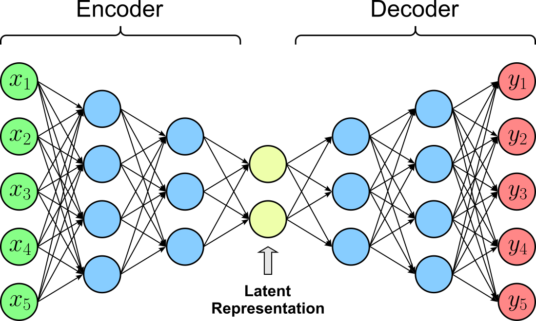
The most fundamental neural network architecture that implements this "encoder-decoder reconstruction" paradigm is the so-called autoencoder. In principle, the encoder and decoder architectures of an autoencoder can be chosen entirely independently and composed of arbitrary, mismatched model types depending on the data's format — for instance, paired with a custom loss function, a Convolutional Neural Network (CNN) could theoretically encode an image into a latent vector which a Recurrent Neural Network (RNN) then decodes into a textual description. In practice, however, they are almost always structurally symmetric mirrored counterparts utilizing the same core layer types, such as MLP-to-MLP, CNN-to-CNN, or RNN-to-RNN. This structural symmetry is a highly practical design choice: using the same type of architecture for both halves ensures that the decoder possesses the exact mathematical capacity and inductive biases required to invert the specific spatial, temporal, or hierarchical features extracted by the encoder, making the reconstruction optimization much more stable and efficient.
As an example, the figure below shows a simple MLP-to-MLP autoencoder to reduce the dimensionality of our demo dataset from $5$ down to $2$ dimensions. The encoder MLP first maps the $5$ input features down to $4$, then $3$, and finally to $2$. The decoder "reverses" this mapping, bringing the $2$ feature back up to $3$, $4$, and finally $5$ outputs. During training, the model learns to reconstruct the inputs such that $y_i \approx x_i$ for all $i \leq i \leq 5$.
Let's actually implement and train this model. The class MLPAutoencoder in the code cell below implements this simple autoencoder using PyTorch. By default, the class assumes an input size of $5$ to match the number of features of our demo dataset, and a latent size of $2$. However, both input and latent size are arguments of the constructor and can be set as needed. While not fundamentally needed, we "organize" the layers of the encoder and decoder into respective instances of the nn.Sequential class. This makes it later easy to reduce the dimensionality of any input by just using the encoder.
class MLPAutoencoder(nn.Module):
    def __init__(self, input_size=5, latent_size=2):
        super().__init__()

        # Encoder: 5 -> 4 -> 3 -> 2
        self.encoder = nn.Sequential(
            nn.Linear(input_size, 4),
            nn.ReLU(),
            nn.Linear(4, 3),
            nn.ReLU(),
            nn.Linear(3, latent_size),
        )

        # Decoder: 2 -> 3 -> 5
        self.decoder = nn.Sequential(
            nn.Linear(latent_size, 3),
            nn.ReLU(),
            nn.Linear(3, 4),
            nn.ReLU(),
            nn.Linear(4, input_size)
        )

    def forward(self, x):
        z = self.encoder(x)
        return self.decoder(z)
To train the autoencoder on our demo dataset we first have to convert the feature matrix X into corresponding PyTorch tensors. We also make use of the TensorDataset and DataLoader classes of PyTorch. While not really needed, using both classes, even for simple examples, is considered best practice because they provide a clean, scalable, and consistent pipeline for handling data. TensorDataset conveniently bundles input features and targets together, while DataLoader automatically manages batching, shuffling, parallel loading, and iteration over the dataset. This keeps training code modular and easy to extend later when moving from demo examples to larger real-world datasets. It also ensures that the same training loop structure can be reused across projects, improving readability, maintainability, and reproducibility.
X_tensor = torch.tensor(X, dtype=torch.float32)

# Create dataset and data loader instances
dataset = TensorDataset(X_tensor, X_tensor)
loader = DataLoader(dataset, batch_size=100, shuffle=True)
Apart from creating an instance of our autoencoder class, we also need to define a suitable loss function as well as an optimizer. The MSELoss (Mean Squared Error) is a suitable loss function for many autoencoders because the model's objective is to reconstruct the input as accurately as possible. MSE measures the average squared difference between the original input and the reconstructed output, encouraging the network to produce reconstructions that are numerically close to the input.
# Create model
model = MLPAutoencoder()
# Create criterion (i.e., loss function)
criterion = nn.MSELoss()
# create optimizer
optimizer = optim.Adam(model.parameters(), lr=1e-3)
We are now ready to train the model. Training an autoencoder typically requires many epochs because the network must simultaneously learn both a compact latent representation of the data and an accurate reconstruction of the original input. Unlike simple supervised tasks with direct target labels, the model needs time to gradually discover meaningful patterns, structures, and feature relationships within the data while minimizing reconstruction error. Since the encoder and decoder are optimized together, convergence can be slower, especially for high-dimensional or complex datasets, making longer training necessary for the latent space and reconstructions to become stable and useful. Thus even, for our demo dataset, let's train the model for $5,000$ epochs.
num_epochs = 5000

for epoch in tqdm(range(num_epochs)):
    for x_batch, _ in loader:
        x_recon = model(x_batch)
        loss = criterion(x_recon, x_batch)
        ### Pytorch magic! ###
        optimizer.zero_grad()
        loss.backward()
        optimizer.step()
100%|███████████████████████████████████████████████████████████████████████████████████████████████████| 5000/5000 [00:19<00:00, 261.28it/s]
We can now use the trained model to reduce the dimensionality of our demo dataset once again from the original $5$ features down to $2$ new features by using only the encoder of the autoencoder model. After that, we can use the plot_2d_projection() to plot the data samples in the projected space.
with torch.no_grad():
    X_autoenc = model.encoder(X_tensor).numpy()

plot_2d_projection(X_autoenc)

Important: Like before, the actual result of the training and dimensionality reduction is the relevant where, since we only work with small demo dataset with no meaningful semantic. The whole purpose of the model implementation and training was to showcase a minimal working example to better appreciate the fundamental idea behind autoencoders.
Beyond basic MLP-based autoencoders, neural networks reduce data dimensions based on the data's structure and the final goal. For images and sequential data, Convolutional Autoencoders (CAEs) and LSTM/RNN Autoencoders replace dense layers with convolutions or recurrent cells to preserve spatial hierarchies and temporal dependencies while keeping parameter counts low. If the data is interconnected—like a social network or molecular structure—Graph Autoencoders (GAEs) compress the data by mapping node features and network topology into a low-dimensional space.
When the goal shifts from simple reconstruction to structuring the latent space itself, Variational Autoencoders (VAEs) and Contrastive Networks (Siamese/Triplet) are the industry standards. VAEs introduce probability distributions to create a smooth, continuous latent space ideal for generative tasks and anomaly detection. Meanwhile, Siamese and Triplet networks bypass data reconstruction entirely; they train on contrastive loss to map data into a metric space where similar items are geometrically close together and dissimilar items are pushed far apart, making them highly effective for similarity search and clustering.
Summary
Dimensionality reduction refers to a collection of techniques used to reduce the number of variables or features in a dataset while preserving as much useful information as possible. As modern datasets often contain hundreds, thousands, or even millions of features, working directly with high-dimensional data can become computationally expensive and difficult to analyze. High dimensionality may also introduce noise, redundancy, and overfitting, a phenomenon commonly associated with the "curse of dimensionality". By reducing the number of dimensions, machine learning models can often train faster, generalize better, and become easier to interpret and visualize.
Dimensionality reduction techniques are commonly grouped into two major approaches: feature selection and feature extraction. Feature selection methods aim to identify and retain only the most relevant original features from the dataset while discarding uninformative or redundant ones. Examples include filter methods based on statistical tests, wrapper methods using model performance, and embedded methods such as Lasso regularization or tree-based feature importance. These techniques preserve the original meaning of the selected variables, which can improve interpretability.
Feature extraction methods, in contrast, create entirely new lower-dimensional representations by transforming or combining the original features. These methods attempt to capture the most important structure or variance within the data in a compressed form. Classical approaches include Principal Component Analysis (PCA), Linear Discriminant Analysis (LDA), and manifold learning techniques such as t-SNE or UMAP. More advanced neural network-based approaches include autoencoders, variational autoencoders, and contrastive representation learning models. Feature extraction is especially powerful for complex data types such as images, audio, text, and high-dimensional scientific data.
Learning about dimensionality reduction is important because it is a foundational tool in modern data science and machine learning. It enables you to handle large and complex datasets more effectively, improve model performance, reduce storage and computational costs, and gain deeper insights into hidden patterns within the data. Since different dimensionality reduction methods make different assumptions and offer different trade-offs between interpretability, compression, and performance, understanding these techniques helps practitioners choose appropriate approaches for real-world applications across many domains.