Disclaimer: This Jupyter Notebook contains content generated with the assistance of AI. While every effort has been made to review and validate the outputs, users should independently verify critical information before relying on it. The SELENE notebook repository is constantly evolving. We recommend downloading or pulling the latest version of this notebook from Github.

Logit Distillation

Logit distillation is a form of transfer learning in which a smaller or simpler student model learns to imitate a larger and more capable teacher model by training directly on the teacher's logits, i.e., the raw, pre-softmax outputs. Although logit distillation can be applied to virtually all kinds of machine learning models, it has become especially popular for efficiently and effectively training small large-language models (LLMs). Modern LLMs are extremely large and expensive to train from scratch, but with logit distillation, a small student can inherit much of the linguistic competence, reasoning ability, and output structure of a large teacher at a fraction of the compute cost. This has made distillation a core technique behind many "compact" LLMs that provide strong performance while running on modest hardware.

The basic idea of logit distillation is to train the student not only to predict correct labels but also to replicate the soft output distribution of the teacher. The teacher's logits reveal which alternative outputs are plausible and by how much. This kind of information is completely lost when using one-hot labels. During training, the student minimizes a combination of standard cross-entropy with ground-truth labels and a distillation loss (often KL divergence) comparing its logits to the teacher's logits. A temperature parameter is commonly applied to soften the distributions, making the teacher's knowledge easier to mimic. By learning from these richer signals, the student model can approximate the teacher’s function more faithfully than it could by relying on hard labels alone. This often results in better generalization, smoother decision boundaries, and significantly improved performance for small models, especially in natural language tasks.

This notebook begins by introducing logit distillation on a conceptual level, explaining how a smaller student model can learn from the raw output logits of a larger teacher model. We will briefly discuss why logits provide a richer learning signal than hard labels, how this approach fits into the broader family of transfer-learning techniques, and why it has become especially important for training efficient yet capable small LLMs.

After building this conceptual foundation, the notebook will walk through a complete hands-on example using PyTorch. We will load a pretrained large language model as the teacher, set up a smaller model as the student, and implement the full distillation workflow—including generating teacher logits, computing the distillation loss, and optimizing the student model. By the end, you’ll have a clear understanding of both the theory and the practical code involved in performing logit distillation for LLMs.

Setting up the Notebook

Make Required Imports

This notebook requires the import of different Python packages but also additional Python modules that are part of the repository. If a package is missing, use your preferred package manager (e.g., conda or pip) to install it. If the code cell below runs with any errors, all required packages and modules have successfully been imported.

import sys
import pandas as pd
import torch
import torch.optim as optim
import torch.nn.functional as F
from torch.utils.data import Dataset, DataLoader

from transformers import GPT2Config, GPT2LMHeadModel
from transformers import AutoModelForCausalLM, AutoTokenizer

from src.utils.compute.gpu import *
from src.utils.data.files import *

Download Required Data

Some code examples in this notebook use data that first need to be downloaded by running the code cell below. If this code cell throws any error, please check the configuration file config.yaml if the URL for downloading datasets is up to date and matches the one on Github. If not, simply download or pull the latest version from Github.

movie_reviews_zip, target_folder = download_dataset("text/corpora/reviews/movie-reviews-imdb.zip")

File 'data/datasets/text/corpora/reviews/movie-reviews-imdb.zip' already exists (use 'overwrite=True' to overwrite it).

We also need to decompress the archive file.

movie_reviews = decompress_file(movie_reviews_zip, target_path=target_folder)

print(movie_reviews)

['data/datasets/text/corpora/reviews/movie-reviews-imdb.txt']

Checking & Setting Computing Device

PyTorch allows to train neural networks on supported GPU to significantly speed up the training process. If you have a support GPU, feel free to utilize it. However, for this notebook it's certainly not needed as our dataset is small and our network model is very simple. We provide an auxiliary method to automatically select the best device. It checks if a supported GPU is available and if so, uses it as the preferred device.

# Select preferred device (GPU, if available; CPU otherwise); you can enfore the use of the CPU
DEVICE = select_device(force_cpu=False)

print("Available device: {}".format(DEVICE))

Available device: cuda:0

Preliminaries

Before checking out this notebook, please consider the following:

• Logit distillation (or more generally: knowledge distillation) is a general approach to train machine learning models. However, in this notebook we focus on training LLMs since knowledge distillation has become particularly popular is this area, and we use this context for our practical example. Still, keep in mind that knowledge distillation is not limited to LLMs!

• This notebook is for education and not to build a state-of-the-art LLM. Not only is the dataset very small it also stems for a single domain: movie reviews. Also, we use the GPT-2 "Small" model as a teacher which is far from a state-of-the-art LLM. But again, our focus is in understanding and clarity not on the model quality.

• While not strictly required, we recommend the presence of a GPU to speed up the training. However, any more modern consumer GPU supported by the PyTorch library should be fine. Even for the full training mode, the default parameters are chosen that the training will not require more than 10 GB of VRAM; with 16GB slowly becoming the standard even for consumer GPUs. However, to stay below 10 GB of memory, the batch size is rather small

• You can run the notebook in different modes where the choice of the mode affects the number of movie reviews used for training. We recommend first using only 1,000 reviews (`mode = "tiny") to see how long the training of the model for individual epochs will require. If everything is working you can increase the dataset size by changing the mode.

#mode = "tiny"  # 1,000 reviews
mode = "small" # 10,000 reviews 
#mode = "full"  # 100,000 reviews

---

Logit Distillation Explained

Many modern machine learning models — especially large neural networks and LLMs — are often over-parameterized. This over-parameterization is useful during training because it helps models fit complex patterns, explore large hypothesis spaces, and achieve strong generalization. However, once trained, these large models are often far more complex than necessary for the specific task or dataset they need to perform on (e.g., a customer chatbot for a banking application). In many practical applications, a smaller model could produce comparable outputs at a fraction of the computational cost, memory footprint, and latency. Despite this, training even a compact model from scratch still requires substantial compute, large datasets, and long training times.

On the other hand, we already have much larger foundation models that "know" language. So why not utilize this knowledge? This is where knowledge distillation becomes valuable. Instead of training a small model independently, distillation allows it to learn directly from an already-trained larger model. By imitating the behavior of the large model the smaller model can inherit much of the teacher's competence without needing the full training pipeline or dataset scale. This dramatically reduces the resources required to produce a high-performing small model, while preserving much of the accuracy and generalization power of the original. As a result, knowledge distillation has become a key strategy for deploying efficient and capable models, particularly in environments where compute, memory, or latency are constrained.

Overview & Basic Idea

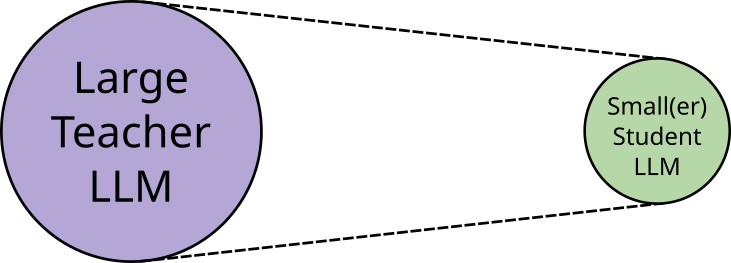
The figure below illustrates on a very high level the basic idea of knowledge distillation in the context of LLMs: take a large pretrained model which performs very well, and transfer or "distill" its knowledge into a (much smaller) model. The "knowledge" that gets transferred is not literal facts or memorized data, but the teacher model's behavior &mdash, that is, its soft probability distributions, reasoning tendencies, and implicit structure of language — rather than explicit facts. These soft targets or soft labels reveal which alternatives are plausible, how confident the teacher is, and how it organizes semantic and syntactic relationships. By training on the teacher's outputs, the student picks up the teacher's inductive biases, heuristics, and task-specific patterns, allowing it to imitate the teacher’s style of reasoning and decision-making even with far fewer parameters.

Knowledge distillation is not a single method but a general concept, and different ways to implement this concept exist. While practical implementation are often hybrid and can differ in many important or subtle details, knowledge distillation can broadly be categorized into three approaches:

• Response distillation uses a teacher model to automatically generate annotations for an unlabeled dataset, allowing the student model to be trained without manual labeling, for example, by having the teacher LLM answer questions that form the training data. It is easy to implement, works in a black-box fashion through APIs, and generally yields high-quality labels if the teacher is strong. However, generating large numbers of annotations can be costly, teacher outputs lack the nuanced information found in logits (making the student less creative or flexible), and the method cannot produce accurate labels for highly domain-specific data the teacher was never trained on. In short, we simple use the teacher model to annotate and unlabeled dataset to train the student model.

• Logit distillation — the focus of this notebook — trains the student model to mimic the teacher model by comparing their logits rather than final text responses, which makes the method both more informative and easier to optimize. In principle, this can be done without labeled data by minimizing a distillation loss (e.g., KL divergence) between teacher and student logits, though this makes evaluation difficult and heavily depends on teacher quality. When ground-truth labels are available, logits distillation can be combined with the standard student loss, offering more stable training and easier evaluation but adding complexity due to the need to balance both losses and manage potential conflicts when the teacher's predictions diverge from the labeled data, especially for examples outside the teacher's training distribution. As long as it is possible to logits as the output from the teacher, logit distillation is still a black-box approach like response distillation

• Feature distillation extends beyond matching the teacher's outputs by training the student to replicate the teacher's internal representations, providing a deeper and richer supervision signal often used alongside logit distillation. However, this approach adds significant complexity because the student is typically much smaller, making it nontrivial to align layers or activations between the two models; for example, a student with fewer or narrower Transformer layers must be mapped to corresponding teacher layers, often requiring strategies like layer selection, learnable projections, or feature pooling to compute a meaningful feature-level loss. Of course, since we now need access to outputs of internal layers, feature distillation inherently assumes white-box access to the teacher model's architecture and parameters.

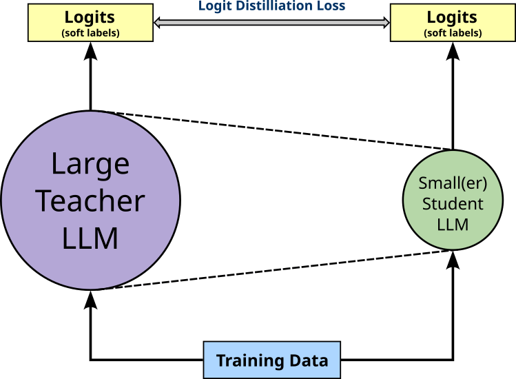
With our focus on logit distillation here, the figure below illustrates the basic idea of training a student model using this approach. More specifically, for variant of logit distillation, we do not need labeled training data since we are only using the logit distillation loss to train the student such that its output mimics the output of the teacher.

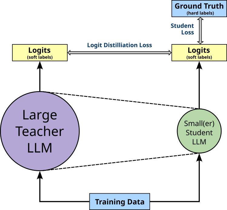
However, in practice, knowledge distillation is often implemented using labeled training data. This means that the training still involves minimizing the student loss, i.e., the loss computed on the students output compared to the ground-truth labels provided by the dataset. Again, the figure below illustrates this setup of training the student model using both the distillation and the student loss.

Since logit distillation allows training the student in a black-box fashion without access in internals of the teacher model, its implementation is rather straightforward. In fact, compared to the standard training setup of an LLM, the only addition is the integration of the distillation loss. So let's see how this can be done and why this is such a promising idea.

Soft Labels vs Hard Labels

When training an LLM on the next-word prediction task using a labeled dataset (and without knowledge distillation) the ground-truth labels (i.e., the target tokens) specify a single correct next token. For example, if a training sample contains the sequence "Last night, I watched a great movie", with respect to the sequence "Last night, I watched a great", the word "movie" is considered the only correct prediction. These so-called hard labels carry no information about alternative possibilities: the model is pushed to place all probability mass on the correct token and zero on everything else. For our example sequence, this includes words such "show", "episode", or "film", which are arguably also good predictions.

The standard loss function when working with hard labels is the Cross Entropy loss $\mathcal{L}_{\text{CE}}$ as defined as follows:

$$\large \mathcal{L}_{hard} = \mathcal{L}_{\text{CE}}(\hat{\mathbf{y}}, \mathbf{y}) = - \sum_{i=1}^{C} y_i \log{(\hat{y}_i)} $$

where $\hat{\mathbf{y}}$ is the predicted output vector in terms of the Softmax probabilities across the set of all classes of size $C$, $\mathbf{y}$ is the hard labels in the form of a one-hot vector with a $1$ at the index representing class $i$; $\hat{y}_i$ and $y_i$ are the individual Softmax labels and hard label for Class $i$ respectively. In the context of training an LLM on the next-word prediction class:

• the set of classes $C$ represents the vocabulary of unique tokens,
• $\hat{y}_i$ represents the output probability of the $i$-th token, $and$
• $y_i$ is either $0$ or $1$ — hard label! — indicating of the $i$-th token is the ground-truth label ($1$) or not ($0$).

Since $y_i\in \{0, 1\}$ and only $1$ for a single token across the whole vocabulary, $\mathcal{L}_{\text{CE}}(\hat{\mathbf{y}}, \mathbf{y})$ only depends on the output probability $\hat{y}_i$ for the $i$-th token. This means that during training, the goal is to maximize the probability of only this single target word — and making no additional distinctions between bad or possible good alternative tokens.

In contrast, soft labels, are probability distributions over all possible next tokens, typically produced by a larger teacher model in knowledge distillation. Instead of saying "the next token must be movie" for our example, a soft label might say: $movie: 0.025$, $show: 0.020$, ... $nice: 0.004$, etc. for all words in the vocabulary. This distribution encodes richer information about uncertainty, similarity between tokens, and linguistic structure. Soft labels therefore give the student model a more nuanced training signal, helping it learn smoother decision boundaries, generalize better, and sometimes require less data compared to training only with hard labels. The figure below illustrates the difference between hard and soft labels for our example where out train sample is "Last night, I watched a great movie" and we want to predict the word "movie" given the previous sequence of words.

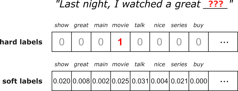
Again, the size of both hard and soft label vectors reflect the size of the vocabulary, and in both cases all vector elements sum up to one — which is obvious in case of the one-hot encoded hard labels. Notice also that the soft labels we get from the teacher model may not give "movie" the highest probability. In other words, there is no reason to assume why the teacher model — even if it is highly accurate — would predict as next word the one given by the training sample.

As the name suggests, logit distillation uses logits, i.e., the pre-Softmax outputs of the student and teacher model, which again are just vectors of the size of the vocabulary. In the following, let $\mathbf{z}^s$ denote the logit output vector of the student model and $\mathbf{z}^t$ the logit output vector of the teacher model. The overall goal of logit distillation is now to update the parameters of the student model such that its output $\mathbf{z}^s$ becomes for similar to the output of the teacher model $\mathbf{z}^t$ for the same input sequence. This means that we need to define a loss function that quantifies the difference between $\mathbf{z}^s$ and $\mathbf{z}^t$. The are two basic approaches to implement such a loss function: using the Kullback–Leibler (KL) divergence or the Mean Squared Error (MSE) loss. Let's look at both of them in detail.

KL Divergence Loss

The seminal paper of knowledge distillation "Distilling the Knowledge in a Neural Network" uses the KL divergence for the knowledge distillation loss. For discrete probability distributions, the KL divergence $KLD$ between to distribution $\mathbf{p}$ and $\mathbf{q}$ is defined as:

$$\large KLD(\mathbf{p}, \mathbf{q}) = \sum_{i} \mathbf{p}_i \cdot \log{\left( \frac{\mathbf{p}_i}{\mathbf{q}_i} \right)} $$

Intuitively, the KL divergence quantifies the information lost when approximating the true distribution $\mathbf{p}$ with an assumed distribution $\mathbf{q}$. We can also say that it quantifies the extra amount of information (e.g., in terms of bits when using $\log_2$) you need because you are pretending the world looks like $\mathbf{q}$ when the true pattern is $\mathbf{p}$. If $\mathbf{q}$ assigns low probabilities to outcomes that happen often under $\mathbf{p}$, the surprise and therefore the KL divergence will be large. If $\mathbf{q}$ matches $\mathbf{p}$ closely, there is very little extra surprise, and the KL divergence approaches zero. In knowledge distillation, $\mathbf{p}$ is the teacher's output distribution, and $\mathbf{q}$ is the student's output distribution: We want the student to imitate the teacher, so we measure how much extra "surprise" we would get if we used the student's predictions ($\mathbf{w}$) to model the teacher's predictions ($\mathbf{p}$).

Since $\mathbf{p}$ and $\mathbf{q}$ need to proper distributions, we first need to convert our logit outputs $\mathbf{z}^s$ and $\mathbf{z}^t$ accordingly. As usual, we can use the Softmax function to convert logits into probabilities. The only common extension is to include of a temperature $\tau$ controls how sharp or smooth the probability distribution becomes when converting logits to probabilities with Softmax:

• High temperature ($\tau > 1$): The logits are divided by a larger number, making them closer together. The Softmax output becomes softer and the differences between classes shrink and the resulting probability distribution is more spread out or "flatter".

• Low temperature ($\tau < 1$)): The logits are divided by a smaller number, exaggerating their differences. The Softmax output becomes sharper, pushing the distribution closer to a one-hot vector.

• Temperature $\tau = 1$ matches the standard Softmax function.

In simple terms, the temperature $\tau$ controls how much the model's confidence is smoothed or amplified, typically helping the student learn more nuanced information when using higher temperatures in knowledge distillation. More formally, we can define the Softmax output for $\mathbf{p}_i$ and $\mathbf{q}_i$ as follows:

$$ \begin{align} \large \mathbf{p}_i &= \large\frac{e^{(\mathbf{z}_i^t/\tau)}}{\sum_j^C e^{(\mathbf{z}_j^t/\tau)}} \\[1em] \large \mathbf{q}_i &= \large\frac{e^{(\mathbf{z}_i^s/\tau)}}{\sum_j^C e^{(\mathbf{z}_j^s/\tau)}} \end{align} $$

For the complete distributions, we can therefore write $\mathbf{p} = softmax(\mathbf{z}^t, \tau)$ and $\mathbf{q} = softmax(\mathbf{z}^s, \tau)$. Again, notice that we use the teacher logits $\mathbf{z}^t$ to compute $\mathbf{p}$ and the student logits to compute $\mathbf{q}$. Thus, we can no define the distillation loss using out soft labels with respect to all $N$ training samples based on the KL divergence as:

$$\large \mathcal{L}_{soft} = \frac{1}{N}\sum_{k}^{N} KLD(\mathbf{p}^{(k)}, \mathbf{q}^{(k)}) $$

where $\mathbf{p}^{(k)}$ and $\mathbf{q}^{(k)}$ are the teacher and student output distributions for the $k$-th training sample.

MSE Loss

A common alternative to using the KL divergence in knowledge distillation is to directly apply the Mean Squared Error (MSE) loss to the raw logits produced by the teacher and student models. This approach bypasses the softmax operation entirely, avoiding the additional complexity introduced by probabilities, temperature scaling, or normalization. Instead, the student is encouraged to regress toward the teacher's pre-softmax output values, which often contain richer information about class relationships, relative confidence levels, and the teacher's internal decision boundaries. Since logits can encode subtle structures that softmax probabilities may wash out, aligning the student to the teacher at the logit level can sometimes lead to more stable or effective training.

Given our two logit outputs $\mathbf{z}^t$ and $\mathbf{z}^s$ from the teacher and student model, the MSE is defined as follows:

$$ \begin{align} \large MSE(\mathbf{z}^t, \mathbf{z}^s) &= \large\frac{1}{C} \sum_{i}^{C} \left( \mathbf{z}^t_{i} - \mathbf{z}^s_{i} \right)^2\\[1em] &= \large \frac{1}{C}\lVert \mathbf{z}^t - \mathbf{z}^s \rVert^2_2 \end{align} $$

Again, $C$ is the number of classes representing the size of both output vectors $\mathbf{z}^t$ and $\mathbf{z}^s$. This gives us now an alternative way to define the loss function using soft labels as the average MSE across all $N$ training samples:

$$\large \mathcal{L}_{soft} = \frac{1}{N}\sum_{k}^N \large MSE((\mathbf{z}^t)^{(k)}, (\mathbf{z}^s)^{(k)}) $$

where $(\mathbf{z}^t)^{(k)}$ and $(\mathbf{z}^s)^{(k)}$ are the teacher and student logit outputs of the $k$-the training sample.

KLD vs MSE Loss: Pros & Cons

Having these to alternatives of computing the soft loss between the teacher and student logits, the obvious question is which to choose in practice. The key difference between using KL divergence and MSE lies in what each loss function actually compares. KL divergence operates on probability distributions, meaning both teacher and student logits must first be passed through a softmax (typically with temperature scaling). As a result, KL-based distillation encourages the student to match the relative probability structure of the teacher, i.e., how the teacher distributes confidence across all tokens. In contrast, MSE operates directly on the raw logits, without converting them into probabilities. This means MSE encourages the student to regress toward the teacher's raw score values, preserving fine-grained differences that softmax may obscure.

KL divergence has the advantage of being theoretically grounded in information theory: it measures how much information is lost when the student approximates the teacher's probability distribution. Because it focuses on relative logit differences rather than absolute values, KL distillation is often more aligned with the ultimate behavior of autoregressive language models, which make decisions through softmax outputs. However, KL divergence can be sensitive to the temperature hyperparameter, and without proper tuning, gradients can vanish when the teacher's distribution becomes very peaked. It can also be computationally more expensive, since softmax operations must be applied at each training step.

MSE on logits, on the other hand, is simpler and often more stable in practice. Since it avoids the softmax, it reduces numerical complexity and eliminates the need for temperature tuning. This can make training faster and easier to debug. Additionally, because logits carry richer information than probabilities, especially about low-probability classes, MSE can transfer subtle teacher knowledge that the softmax would otherwise compress. However, MSE treats all logit dimensions equally, even though in a language model only the relative differences between logits matter for prediction; absolute logit scales may therefore mislead the student unless the teacher's logits are well-behaved.

Ultimately, the choice between KL divergence and MSE depends on the goal and the characteristics of the models involved. If you want the student to closely match the teacher's decision distribution (and are willing to tune temperatures) KL divergence is often the more principled choice. If you prefer a simpler, more direct, and sometimes more stable regression signal, especially early in training or with limited compute, MSE on logits can be an excellent alternative. Both approaches can yield strong results, and many distillation setups combine them with additional losses to balance their strengths. For example, the paper "Comparing Kullback-Leibler Divergence and Mean Squared Error Loss in Knowledge Distillation" compares the loss function shows that MSE often performs better. However, the evaluation was done in the context of an image classification task, and it is not obvious how these results translate to LLMs.

Total Loss

If we want to train the student using both the hard and soft loss, we need to combine both losses to form the total loss to be minimized during training. While there is no single best way to do this, a very common approach is to compute a balanced loss using a weight term $\alpha \in [0, 1]$ that specifies how much the hard loss and the soft loss contribute to the total loss, which we can define as:

$$\large \mathcal{L}_{balanced} = \alpha\mathcal{L}_{hard} + (1 - \alpha)\mathcal{L}_{soft} $$

If $\alpha = 1$ the total loss only depends on the hard loss and this considering only the standard Cross Entropy loss between the student's prediction and the ground-truth labels. In contrast, if $\alpha = 0$, we completely ignore the ground-truth labels and consider only the distillation loss for training the student model. And a value for $\alpha$ between $0$ and $1$ computes some weighted sum of both hard and soft loss. Later, we will define a function that computes the balanced loss and allows us to flexibly set the value of $\alpha$.

---

Logit Distillation — A Complete Practical Example

Now that we know how logit distillation works, let's go through a concrete example of implementing logit distillation to train an LLM. More specifically, we use the pretrained GPT-2 model as the teacher and guide a compact student model to approximate its behavior on a given dataset. Throughout the rest of this notebook, we walk step-by-step through the full distillation workflow: preparing data, generating teacher logits, defining the distillation loss, and training the student model. The emphasis is on clarity and practical implementation, showing how logit distillation can significantly reduce training cost while still preserving much of the teacher's predictive power. By the end, you will have a clear understanding of how to implement logit distillation in practice and how it can serve as an effective strategy for compressing large language models.

Dataset Preparation

The ACL IMDB (Large Movie Review) dataset is a widely used benchmark dataset for sentiment analysis, introduced by Andrew Maas and colleagues at Stanford in 2011. It contains 50,000 labeled movie reviews** from IMDb, evenly split into 25,000 for training and 25,000 for testing, with an equal number of positive and negative reviews in each split. In addition to the labeled reviews, the dataset includes 50,000 unlabeled reviews, intended to support semi-supervised learning experiments. For training the student model, we do not need the sentiment labels but only the review texts. We therefore already preprocessed the original dataset such that all 100,000 reviews are in a single file, with 1 line = 1 review. This preprocessing included the removal of any HTML tags and line breaks.

For the training, we are following the common idea of treating the entire corpus as a continuous stream of documents, i.e., as one long, uninterrupted sequence of tokens rather than as separate, independent documents. Because document boundaries still matter semantically, many implementations insert special boundary tokens (e.g., [EOS]) to signal the transitions between documents. During training, chunks are drawn such that the model learns from natural text continuity while still being able to infer when one document ends and the next begins. This method helps maintain statistical consistency, supports scalable data pipelines, and aligns with how modern language models (e.g., GPT-style models) are typically trained on web-scale corpora. Thus, assuming $\text{doc}_{i}$ is a list of tokens represents the $i$-th documents, our document stream has the following format:

$$\large \text{doc}_{1} + \text{[EOS]} + \text{doc}_{2} + \text{[EOS]} + \text{doc}_{3} + \text{[EOS]} + \dots $$

In practice, training on web-scale corpora is challenging because these datasets are far too large to fit into memory, making it impossible to load, shuffle, or repeatedly traverse them in the traditional way. Instead, the model must read the data as a continuous stream from disk or distributed storage, which introduces issues such as maintaining efficient throughput, handling document boundaries, and ensuring sufficient randomness without full in-memory shuffling. These constraints force the design of specialized data pipelines that can deliver tokens sequentially while still providing the statistical diversity required for effective language-model training. However, in this notebook, we can ignore these considerations since our dataset is small and fits into memory, making its handling much simpler.

Load Reviews from File

In the setup section of the notebook, we already downloaded the file containing all 100,000 movie reviews. In the following code cell, simply counts the number of reviews by containing the number of each line in the file, just to check if the dataset is complete. Note that we have to write movie_reviews[0] since movie_reviews is a list of files — it just so happens that the list contains only one file.

total_reviews = sum(1 for _ in open(movie_reviews[0]))

print(f"Total number of reviews (1 review per line): {total_reviews}")

Total number of reviews (1 review per line): 100000

Although we have a total 100,000 reviews (each containing multiple sentences), we consider only 10,000 reviews in demo mode to speed up the training. However, you can edit the code cell below to increase or decrease the number of considered reviews. For a first run, we recommend sticking to 10,000 reviews to execute and understand the code.

if mode == "tiny":
    num_considered_reviews = 1_000
elif mode == "small":
    num_considered_reviews = 10_000
else:
    num_considered_reviews = 100_000

num_reviews = min(total_reviews, num_considered_reviews)

print(f"Number of reviews used for training dataset: {num_reviews}")

Number of reviews used for training dataset: 10000

Tokenize & Generate Token Stream

Modern LLMs are trained on documents tokenized with subword tokenizers because these tokenization methods provide a flexible balance between character-level and word-level representations. Natural language contains an enormous vocabulary with many rare words, inflections, and spelling variations that are difficult to model using pure word-level tokenization, which would require an impractically large vocabulary and produce many out-of-vocabulary tokens. Subword tokenizers (e.g. BPE, WordPiece, and SentencePiece) break words into smaller, reusable units, allowing the model to represent any text as a sequence of known symbols while still capturing meaningful linguistic structure.

The benefits of subword tokenization are substantial: it dramatically reduces vocabulary size, ensures coverage of all possible text inputs, and allows the model to share statistical strength across related words through common subword components. This leads to more efficient training, improved generalization to unseen words, and better handling of multilingual or noisy data. By limiting the vocabulary while preserving expressiveness, subword tokenizers enable LLMs to scale to massive corpora without exploding memory requirements or losing linguistic nuance.

Since our teacher model is GPT-2, we also need to use the corresponding pretrained GPT-2 tokenizer because the model was trained on text that was tokenized in a very specific way. The tokenizer defines the mapping from raw text to token IDs, including how words are split into subwords, special tokens used, and the exact vocabulary. If a different tokenizer were used, the input IDs would not match the representations the model expects, leading to incorrect embeddings and poor or nonsensical outputs. Essentially, the tokenizer and model must be aligned to ensure that the model interprets text in the same way it saw during pretraining. The GPT-2 tokenizer uses Byte-Pair Encoding (BPE) and has a vocabulary size of $50,257$.

To load the pretrained GPT-2 tokenizer, we can use the AutoTokenizer class Hugging Face Transformers library. This class is a high-level interface that automatically selects the appropriate tokenizer for a given pretrained model, abstracting away the need to know the specific tokenizer class. The from_pretrained method is used to load a tokenizer that has already been trained on a specific model's vocabulary and tokenization rules, either from the Hugging Face model hub or a local path. The code cell below uses the class and method to load the GPT-2 tokenizer.

model_name = "gpt2"

tokenizer = AutoTokenizer.from_pretrained(model_name)

Recall that for our document stream, we need to indicate when one movie review ends and another review starts using some [EOS] (end-of-sequence) token. However, we cannot simply define our own unique token but must use a token that is known to the tokenizer, i.e., the token is part of the existing vocabulary. Most tokenizers include a small set of special tokens to indicate the end of a sequence, the beginning of a sequence, padding tokens, masked tokens, etc. — all depending on the data and learning task.

We can check the special_tokens_map of the GPT-2 tokenizer which special tokens it supports:

tokenizer.special_tokens_map

{'bos_token': '<|endoftext|>',
 'eos_token': '<|endoftext|>',
 'unk_token': '<|endoftext|>'}

We can see that the GPT-2 tokenizer recognizes only one special token: <|endoftext|>. Since GPT-2 was also trained on a document stream, we only need a single token acting as a separator between documents, which could be either the [EOS] or [BOS] token. The GPT-2 tokenizer also does not require a dedicated [UNK] (unknown) token, since BPE just tokenizes unknown words into known subwords or even just characters, if needed. Let's define this <|endoftext|> token as a constant for creating our document stream.

EOS_TOKEN_GPT2 = "<|endoftext|>"

With the tokenizer, we can now go through all movie reviews (or the maximum number of reviews specified) and tokenize them; see the code cell below. Notice that the preprocess each review before tokenizing by removing any newline characters, converting all words to lowercase, and adding the special [EOS] token at the end.

Lowercasing all words can be very useful when working with smaller datasets because it significantly reduces the size of the vocabulary the model needs to learn. In a small corpus, many words appear only a handful of times, and treating uppercase and lowercase forms as separate tokens (e.g., "Movie" vs. "movie") further fragments the data. By converting everything to lowercase, the model encounters each word more frequently, allowing it to learn better embeddings and stronger statistical patterns from limited examples. This makes training more stable and reduces the risk of overfitting to infrequent capitalized variants.

Additionally, the goal in many educational or exploratory projects is to understand the mechanics of training sequence models and not to capture subtle linguistic nuances such as proper noun capitalization. Lowercasing simplifies preprocessing, reduces noise, and helps the model focus on learning the core structure of the language rather than expending capacity on orthographic variations. For small-scale experiments, this trade-off is highly beneficial: you get cleaner data, faster training, and more reliable results without sacrificing the insights the project aims to teach.

tokens = []

with open(movie_reviews[0]) as file:
    for idx, review in enumerate(tqdm(file, total=num_reviews, leave=False)):
        if idx >= num_reviews:
            break
        tokens.extend(tokenizer.encode(f"{review.strip()} {EOS_TOKEN_GPT2}", truncation=True, max_length=sys.maxsize))

print(f"Total number of tokens: {len(tokens)}")

Total number of tokens: 2880982

Create Dataset and DataLoader

In PyTorch, the Dataset class is an abstraction that defines how data is accessed and preprocessed for training. It provides a consistent interface to load individual samples and their labels through the methods __len__() and __getitem__(). This allows you to wrap any type of data (text, images, tabular data, etc.) into a standardized format that PyTorch models can easily consume. The DataLoader class then builds on top of this by handling the efficient batching, shuffling, and parallel loading of data samples from a Dataset. It automatically groups multiple samples into mini-batches and can use multiple worker processes to load data in parallel, ensuring that the GPU remains fully utilized during training.

For creating our Dataset instance, recall that GPT-style LLMs are trained based on the next-word prediction task — given a sequence of words which is the next likely word to follow. The figure below shows the required training setup for the Transformer decoder. The target sequence is (almost) the same as the input sequence, only 1 token shifted to the left. Note that the dashed line represents the causal masking where the prediction of a token only depends on preceding tokens but not "future" tokens — recall that the decoder processes all tokens in parallel during training, so we need to mask the attention between a token and all tokens preceding it.

Of course, we cannot give the whole sequence of tokens to the model at once. When training LLMs, the context size, i.e., the number of tokens the model can attend to at once, is typically fixed to a maximum value due to both computational and architectural constraints. Transformer models compute attention across all token pairs within a sequence, which scales quadratically with sequence length in both memory and computation cost. This means that doubling the context size roughly quadruples the resources required per training step. To make training feasible on available hardware, a practical upper bound (e.g., 512, 1024, or 4096 tokens) is chosen so that the model can learn meaningful dependencies without exhausting GPU memory or dramatically slowing training.

We therefore have to feed the model all tokens in chunks. In this notebook, we use a common sliding window approach that forms a chunk of a fixed size. More specifically, we use a sliding window with a 50% overlap — see the example in the figure below. In this simple example, the context size is 6 tokens, meaning that an overlap of 50% means that the last 3 tokens of the current chunk will be the first 3 tokens of the next chunk.

The class GPT2TextDataset in the code cell below implements the sliding window approach as a custom Dataset class. The max_len parameters specify the maximum context size, and the optional stride parameter specifies by how many tokens the slides window should be moved each time. If stride=None move the window by the whole context size, thus resulting in chunks without overlap. Notice that we return only the input sequences but not the target sequences. This is because we will later use the GPT2HeadeModel class to create the student model. This class performs the shifting of the input sequences by $1$ token to the left to get the target sequences under the hood, so we do not have to worry about that.

class GPT2TextDataset(Dataset):
    def __init__(self, tokens, max_length=128, stride=None):
        self.input_ids  = []
        
        if stride is None:
            stride = max_len

        for i in range(0, len(tokens)-max_length, stride):
            self.input_ids.append(torch.LongTensor(tokens[i:(i+max_length)]))

    def __len__(self):
        return len(self.input_ids)

    def __getitem__(self, idx):
        return self.input_ids[idx]

Let's use our list of all tokens to create an instance of the GPT2TextDataset class. For this, we need to specify the context size, i.e., the maximum length of the input sequences. When training an LLM, the context size (or context window) refers to the maximum number of tokens the model can attend to at once through its self-attention mechanism. This determines how far back in the text the model can directly "look" when predicting the next token. For example, if the context size is $1,048$ tokens, the model can condition its predictions on at most those $1,048$ previous tokens, regardless of how long the full document is.

In principle, the context size is not a direct hyperparameter for knowledge distillation tasks, since the context size does not determine the size or complexity of the model — which depends on the number of layers, the width of each layer (hidden dimension), and the number of attention heads. These architectural choices determine the total number of parameters, compute cost, and representational capacity. The context size only affects the shape of the training data and the compute per forward pass (since attention scales with sequence length), but it does not change the learned weights or the overall architecture.

However, there are two considerations when setting the context_size parameter in the code cell below

• The context size of the GPT-2 model is $1,024$ tokens, and it cannot use a larger context during inference because it relies on learned absolute positional embeddings. Unlike modern models that often use relative encodings (like RoPE or ALiBi) to generalize to longer lengths, GPT-2 was trained with a fixed lookup table (a specific weight matrix) containing exactly 1,024 unique vectors, one for each possible position in the sequence. Consequently, if you attempt to feed the model more than $1,024$ tokens, it physically lacks the trained parameters to represent the position of the $1,025$th token, making inference impossible without truncating the input or fundamentally modifying and retraining the architecture. In short, we cannot set context_size to a value larger than $1,024$.

• While the context size does not affect the model size, it does directly affect the memory requirements for training and inferencing because the attention mechanism scales quadratically with sequence length: for a context window of $N$ tokens, each layer computes an $N\!\times\!N$ attention matrix. During training, as $N$ grows, the model must store larger intermediate representations, gradients, and attention scores, which directly increases GPU memory usage. Longer sequences also increase the amount of activation memory that must be kept for backpropagation, making training significantly more expensive even when the model architecture (number of layers, hidden size) stays the same. Inference requires less memory, but the model still computes an $N\!\times\!N$ attention matrix, the memory requirements still scale quadratically.

By default, we set the context size to $128$ (see below), which is often considered on the lower end for training small LLMs on small datasets. That being said, if you run out of memory when training the student model using logit distillation, you can try further reducing the context size to lower the overall memory footprint.

context_size = 128

dataset = GPT2TextDataset(tokens, max_length=context_size, stride=context_size//2)

Using the dataset instance, we can now also create the data loader instance that handles all the batching and shuffling for us.

loader = DataLoader(dataset, batch_size=32, shuffle=True, drop_last=True)

During training, we can simply use the data loader to iterate over all batches. The code cell below shows the general idea, but only prints the shape of the first batch for illustration purposes. Appreciate that we did nothing to create the batches, which is all managed by the data loader. While using larger batch sizes generally improves efficiency, larger batches also mean larger memory requirements. So again, if needed, you can reduce the batch size to safe memory.

for batch in loader:
    print(batch.shape)
    break

torch.Size([32, 128])

As you should have expected, the shape of a batch is (batch_size, context_size), reflecting the values we have chosen for both parameters.

---

Auxiliary Methods

For the model training and the very crude qualitative evaluation of the model (discussed later), we next define a few auxiliary models for a cleaner code but also support strategies such as checkpointing for training large models in practice.

Compute the Model Size

The overall goal of knowledge distillation is to use a large(r) pretrained teacher model to help train a (much) smaller student model. To allow for some meaningful comparison, we need to somehow quantify the size of a model. Most commonly, the size of machine learning models (incl. LLMs) is measured by the number of parameters because parameters directly represent a model's capacity to learn and store information. Each parameter corresponds to a learned weight that shapes how the model processes inputs and makes predictions, so more parameters generally mean a larger and more expressive function class.

In the method code cell below, the method count_parameters() returns two values: the total number of model parameters as well as the number of trainable parameters (i.e., the number of parameters that get updated during training). To this end, count_parameters() simply utilizes methods provided by PyTorch.

def count_parameters(model):
    n_params = sum(p.numel() for p in model.parameters())
    n_trainable_params = sum(p.numel() for p in model.parameters() if p.requires_grad)
    return n_params, n_trainable_params

Loss Functions

The connection between the student and the teacher model during training happens through the loss function — more specifically, through the loss function computing the soft loss (see above). Since these loss functions are not part of the standard toolbox of PyTorch we have to implement them ourselves. However, the methods provided by PyTorch allow for a direct implementation of the given formulas of both alternatives.

Firstly, the method kl_div_loss() below computes the loss using the Kubler-Leibler (KL) Divergence after applying the softmax to both the teacher and student logits. Notice that we compute the log softmax since the PyTorch method kl_div(p, q, ...) expects p to be log probabilities. By default, the method expects q to be probabilities, but by setting log_target=True we can pass log probabilities here as well. Lastly, the parameter reduction="batchmean" means that the method will sum the KL divergence over all elements in each sample, then average that total over the batch size. This keeps the loss scale consistent regardless of sequence length or number of classes, making the magnitude of the loss more stable when training across different batch sizes.

def kld_loss(student_logits, teacher_logits, temperature=2.0):
    p = F.log_softmax(student_logits / temperature, dim=-1)
    q = F.log_softmax(teacher_logits / temperature, dim=-1)
    return (temperature*temperature) * F.kl_div(p, q, log_target=True, reduction='batchmean')

We saw that a second way to compute the soft loss was to use the raw logits and compute the Mean Squared Error (MSE) between them. Since the PyTorch provides the mse_loss() function out of the box, we can simply define a wrapper method mse_logit_loss() that uses this built-in method to compute the MSE loss between the student and teacher logits.

def mse_logit_loss(student_logits, teacher_logits):
    return F.mse_loss(student_logits, teacher_logits)

Training a Single Epoch

The train_epoch() function performs one full training pass over a dataset while applying knowledge distillation from a larger teacher model to a smaller student model. For each batch of tokenized input sequences, the method runs the student model in training mode and computes the standard causal language-modeling loss, which measures how well the student predicts the next token in the sequence. At the same time, it also runs the teacher model on the same inputs to obtain its logits, which provide a softer, more informative probability distribution over next-token predictions.

To combine these two learning signals, the function computes a weighted sum of two losses: the hard loss (cross-entropy with the true labels) and the soft loss (KL divergence between student and teacher logits). The weighting factor alpha controls how much the student should rely on ground-truth labels versus mimicking the teacher. After calculating the blended loss, the method performs standard PyTorch backpropagation and optimizer steps to update the student model's parameters.

Some additional noteworthy details about the internals of the pretrained model instance:

• GPT-2 is a decoder-only Transformer and already applies a causal mask internally (tokens can't attend to future tokens). However, the model instance still needs an attention_mask to handle padding or masked-out tokens. Since all of our sequences always have the same length, we do not need to mask out any tokens and can simply instantiate the attention mask with all $1$s

• Notice that with labels=input_ids we pass the input sequences as the labels/targets without shifting the sequences $1$ token to the left. This is done internally by the AutoModelForCausalLM. This shifting causes the target sequences to be $1$ token short, the model simply ignores the last token. This does not matter for any practical context size.

def train_epoch(loader, teacher, student, criterion, optimizer, description, alpha=0.5):
    student.train()
    epoch_loss = 0.0
    device = next(student.parameters()).device
    for idx, input_ids in enumerate(tqdm(loader, desc=description, leave=False)):
        # Move current batch to GPU, if available
        input_ids = input_ids.to(device)
        # Compute attention mask since it's mandatory
        attention_mask = torch.ones_like(input_ids)
        # Forward pass + compute (hard) loss
        outputs = student(
            input_ids=input_ids,
            attention_mask=attention_mask,
            labels=input_ids   # causal LM: predict next token
        )
        # Get logit outputs from student and teacher        
        student_logits = outputs.logits
        teacher_logits = teacher(input_ids).logits
        # Compute weighted loss between the hard loss and soft loss
        hard_loss = outputs.loss
        # Compute total loss as balanced loss between hard and soft loss
        loss = criterion(hard_loss, teacher_logits, student_logits)
        # Perform PyTorch magic (backpropagation + parameter updates)
        student.zero_grad()
        loss.backward()
        optimizer.step()
        # Update epoch loss
        epoch_loss += loss.item()
    return epoch_loss

Saving & Loading Checkpoints

Although the goal of knowledge distillation is to train smaller models, it typically still requires a lot of computing resources and training time. To avoid an loss of progress (e.g., in case of a crash), we can use checkpoints A checkpoint in model training is a saved snapshot of the model's state at a specific point during training, typically after a certain number of steps or epochs. It usually includes the model's parameters (weights and biases), the optimizer state (to resume learning with the same momentum and learning rate adjustments), and sometimes metadata like the current epoch or training loss. This allows training to be paused and later resumed from that point without starting over, which is especially important for large models that take days or weeks to train.

While many libraries have built-in support for periodically saving checkpoints, in this notebook, we purposefully use only PyTorch and avoid libraries with a higher level of abstraction. However, saving a checkpoint is very straightforward. The method save_checkpoint() defined in the code cell below takes a model and optimizer instance, as well as the information about the current epoch and epoch loss. The method then combines all required information to resume training into a single object and uses the save() method of PyTorch to save this object to a file.

In PyTorch, the state_dict() object is a Python dictionary that contains all the learnable parameters and persistent states of a model or optimizer. For models, it stores mappings from each layer's name to its corresponding tensor values (like weights and biases). For optimizers, it includes the current state of optimization variables such as momentum buffers and learning rate schedules. This dictionary enables easy saving, loading, and transferring of model and optimizer states, making it central to checkpointing and model deployment. By calling torch.save(model.state_dict()), you can preserve a model's learned parameters, and later restore them with model.load_state_dict(), ensuring the model continues exactly where it left off.

def save_checkpoint(model, optimizer, epoch, loss, path="checkpoint.pt"):
    checkpoint = {
        "epoch": epoch,
        "model_state_dict": model.state_dict(),
        "optimizer_state_dict": optimizer.state_dict(),
        "loss": loss,
    }
    torch.save(checkpoint, path)
    print(f"Checkpoint saved at {path}")

Naturally, the counterpart to saving a checkpoint is loading a save checkpoint, as implemented by the method load_checkpoint() below. Notice that this method also takes in a model and optimizer instance. In other words, the method does not create a model or optimizer but sets the state of both instances as the states read from the checkpoint file. This of course only works if the model and the optimizer have the same "structure" as the model and optimizer used for training. For example, we cannot train a Transformer model with 4 layers and then load its state into a model with more or less layers.

Also, notice the map_location parameter of PyTorch's load() method. This parameter controls how tensors are remapped to devices (like CPU or GPU) when loading a saved model or checkpoint. This is useful when the model was trained on one device but needs to be loaded on another; for example, loading GPU-trained weights onto a CPU-only machine. By specifying map_location='cpu', all tensors are loaded to the CPU regardless of where they were originally saved, while map_location='cuda:0' loads them to the first GPU. It can also take a custom function or dictionary to flexibly remap devices, ensuring model compatibility across different hardware setups and preventing errors caused by unavailable devices.

def load_checkpoint(model, optimizer, path="checkpoint.pt", device="cuda"):
    checkpoint = torch.load(path, map_location=device)
    model.load_state_dict(checkpoint["model_state_dict"])
    optimizer.load_state_dict(checkpoint["optimizer_state_dict"])
    epoch = checkpoint["epoch"]
    loss = checkpoint["loss"]
    print(f"Checkpoint loaded (epoch {epoch}, loss {loss:.4f})")
    return epoch, loss

Generate & Save Example Responses

To see how the student model's performance improves over time, we only perform a naive qualitative evaluation by monitoring how the model will complete an initial prompt after each epoch — instead of a proper evaluation which is very challenging in case of LLMs and beyond the scope of this notebook. To this end, generate_response() encapsulates all the required steps to generate a response for a given prompt, mainly (1) tokenizing the seed prompt and converting the tokens to their unique ideas, (2) pass these token ids to the model to get the generated output token ids in return, and (3) use the tokenizer again to decode the output token ids to a human-readable string.

def generate_response(prompt, tokenizer, model, max_new_tokens=50, do_sample=True, temperature=1.0, top_p=0.5):
    # Get the device where the model is located
    model_device = next(model.parameters()).device
    # Tokenize input
    inputs = tokenizer(prompt, return_tensors="pt", padding=False, truncation=True).to(model_device)
    input_ids = inputs["input_ids"]
    attention_mask = inputs["attention_mask"]
    # Generate continuation
    output_ids = model.generate(
        input_ids=input_ids,
        attention_mask=attention_mask,
        max_new_tokens=max_new_tokens,
        temperature=temperature,
        top_p=top_p,
        do_sample=True,     # enable stochastic sampling
        eos_token_id=tokenizer.eos_token_id,
        pad_token_id=tokenizer.eos_token_id,
    )
    # Decode to string and return generated response
    return tokenizer.decode(output_ids[0], skip_special_tokens=True)

Since we later save some results to file and potentially also save checkpoints, we define a target folder where all files generated as part of this notebook are stored. Of course, you can change the default target folder to match your preference.

folder = create_folder("data/generated/models/knowledge-distiallation-gpt2/")

print(folder)

data/generated/models/knowledge-distiallation-gpt2/

Creating the Models

Teacher Model

As mentioned at the beginning, we are using the GPT-2 model as the teacher. The GPT-2 model is publicly available through Hugging Face's transformers library, making it extremely easy for anyone to load and experiment with. With just a few lines of code — using the from_pretrained method of the AutoModelForCausalLM class — you can download the pretrained weights and model architecture directly from the hub.

GPT-2 is released in several model variants, each differing in size and capacity. These variants share the same overall architecture but scale in depth (number of layers), width (embedding size), and number of attention heads. This allows users to choose a model that fits their compute budget—smaller models run faster and require less memory, while larger models provide stronger performance. The table below provides an overview of the main variants.

Variant	Parameters	Layers	Embedding Size	Attention Heads	Notes
GPT-2 Small	~117M	12	768	12	Default “base” model used in many tutorials
GPT-2 Medium	~345M	24	1024	16	More expressive, but heavier to train and run
GPT-2 Large	~774M	36	1280	20	Significant performance improvement
GPT-2 XL	~1.5B	48	1600	25	Largest publicly released GPT-2 model

In the table above, the GPT-2 Small variant with ~117M parameters is also often called the GPT-2 base model. This is the default and most commonly referenced version of GPT-2. It has 12 layers, a 768-dimensional embedding size, and 12 attention heads. Hugging Face refers to it simply as "gpt2", and it is typically what people mean when they say "GPT-2 base". And this variant is what we will be using as well; see the code cell below. You are welcome to go with a larger variant but keep in mind that this will come with higher memory requirements.

teacher = AutoModelForCausalLM.from_pretrained(model_name).to(DEVICE)

Although the soft loss depends on the logits of both the student and the teacher model, we do not actually want to train the teacher model. To avoid any parameter updates for the teacher model we have to "freeze" it. In PyTorch, we can achieve this by setting param.requires_grad = False for all the model parameters. This tells the autograd engine not to compute gradients for that parameter during backpropagation. We also set the teacher model into evaluation mode with teacher.eval(). This switches the model to evaluation mode, which alters the behavior of certain layers like dropout and batch normalization. In this mode, dropout layers stop randomly zeroing activations, and batch normalization uses running statistics instead of batch statistics, ensuring deterministic and consistent outputs. This is essential when evaluating or generating predictions, so the model's behavior matches how it was intended to operate after training.

for param in teacher.parameters():
    param.requires_grad = False
teacher = teacher.eval()

Let's check the number of (trainable) parameters for the teacher model using our auxiliary method count_parameters().

n_params_teacher, n_trainable_params_teacher = count_parameters(teacher)

print(f"Total number of parameters: {n_params_teacher:,}")
print(f"Number of trainable parameters: {n_trainable_params_teacher:,}")

Total number of parameters: 124,439,808
Number of trainable parameters: 0

The number of trainable parameters is of course $0$ since we just froze the complete model to avoid updating its weights when training the student model.

Notice that we also see ~124M parameters in total, more than the ~117M parameters in the table above. The discrepancy arises from different ways of counting parameters. The often-cited 117M refers to the original GPT-2 Small parameters in the OpenAI paper, which usually counts only the core model weights (transformer layers). When you load the model via Hugging Face in PyTorch, the 124M count includes additional parameters such as the token embeddings and final layer normalization weights, which are part of the full implementation but not always included in the paper's parameter tally.

Models loaded using the transformers library also come with a configuration object that contains all the core information about the model. For example, in the code cell below, we use this configuration object to check the embedding size, the number of layers, and the number of heads — all those match, of course, the values reported in the previous table.

teacher_config = teacher.config

print(f"Embedding size: {teacher_config.n_embd}")
print(f"Number of layers: {teacher_config.n_layer}")
print(f"Number of heads: {teacher_config.n_head}")

Embedding size: 768
Number of layers: 12
Number of heads: 12

We can also qickly see how the model performs on an example prompt by using our generate_response() auxiliary method.

prompt = "The best part of the movie was"

print(generate_response(prompt, tokenizer, teacher))

The best part of the movie was the music, the sound, the way the music was played. It was just so good.

How did you make the film?

I had to make it from scratch. I was working with the director, and I had to get

Keep in mind that the GPT-2 Small model is far from a state-of-the-art language model by today's standards. Modern LLMs are significantly larger, more capable, and trained on far more diverse datasets. However, GPT-2 Small remains a useful and lightweight reference point for educational and experimental purposes. Its modest size means it can run comfortably on typical consumer hardware, making it an accessible option for illustrating core concepts without the complexity or overhead of cutting-edge models.

In this notebook, we intentionally use GPT-2 Small as the teacher to keep the memory footprint, compute requirements, and training time manageable for our logit distillation example. The goal here is not to push performance boundaries, but to provide a clear and practical demonstration of how logit distillation works in principle. By choosing a smaller teacher, we ensure that the entire workflow — from loading the model to generating logits and training the student — remains efficient and reproducible on common setups.

Student Model

When it comes to the student model, we only have two main restrictions. Firstly and most obviously, the student must also be an autoregressive model to match the next-word prediction task. And secondly, the model must work with the same vocabulary. Not only must the logit output $\mathbf{z}^t$ and $\mathbf{z}^s$ match in size, they must also be aligned with respect to the vocabulary. This means that the $i$-th value in both $\mathbf{z}^t$ and $\mathbf{z}^s$ most refer to the same token. The obvious way to ensure this is to simply use the same tokenizer instance for both the teacher and student model.

Apart from that, since logit distillation only relies on both models output, the teacher and the student can "look" quite differently. For example, in principle the student can be an RNN-based model even when the teacher is a Transformer. Distillation does not require teacher and student architectures to match; it only requires that the student can produce outputs in the same format as the teacher so that the distillation loss can be computed. As long as the student RNN can generate logits over the same vocabulary as the Transformer teacher, it can be trained to approximate the teacher's behavior through MSE or KL divergence-based soft losses.

However, several practical challenges arise. Transformer teachers typically produce richer contextual representations due to their self-attention mechanisms, while RNNs rely solely on sequential recurrence, which may limit the student's ability to fully mimic the teacher's long-range dependencies. This mismatch in capacity and inductive bias can make distillation less effective unless the student is adequately sized or supplemented with architectural enhancements such as attention mechanisms or gating. Despite these limitations, cross-architecture distillation such as Transformer-to-RNN remains feasible and has been successfully explored in research when efficiency or deployment constraints prioritize smaller, simpler models.

However, to keep it simple, we go with another GPT-2 model for the student. Note that GPT-2 only refers to the vocabulary size, the pretrained tokenizer, and general Transformer-based architecture — GPT-2 does not refer to any specific size of the model in terms of the token embedding size, the number of attention heads, the number of attention heads, and so on. By choosing a GPT-2 model we can not only use existing classes from the transformers library to create the model, but also our auxiliary method generate_response() for bot the teacher and model.

To define our student model, we use the GPT2Config class of the transformers library. This class defines all the hyperparameters and architectural settings used to construct a GPT-2 model. Instead of hard-coding model dimensions, number of layers, attention heads, vocabulary size, and other internal parameters directly in the code, these values are encapsulated inside a configuration object. This configuration is what the model uses to determine its structure — everything from hidden size and number of transformer blocks to dropout rates, activation functions, and positional embedding settings. In the code cell below, we create a GPT2Config instance using only $1/3$ of the embedding size ($256$ instead of $768$), $1/3$ of the number of attention heads ($4$ instead of $12$), and $1/3$ of the number of layers ($4$ instead of $12$) compared to the teacher model (i.e., GPT-2 Small, by default).

student_config = GPT2Config(
    vocab_size=50257,
    n_positions=128,
    n_ctx=128,
    n_embd=256,
    n_layer=4,
    n_head=4
)

To create the actual model based on this configuration, we can use the GPT2LMHeadModel class. It consists of the standard GPT-2 transformer architecture plus an additional linear output layer (i.e., the "language modeling head") that maps the hidden states to logits over the vocabulary. This design allows the model to predict the next token in a sequence, making it suitable for tasks such as text generation, completion, and autoregressive training. The class handles the forward pass, loss computation (when labels are provided), and all components needed for next-token prediction. Importantly, GPT2LMHeadModel also includes utilities that simplify training and inference. For example, it automatically performs the left-shift of labels required for autoregressive loss computation.

student = GPT2LMHeadModel(student_config).to(DEVICE)

Like for the teacher model, let's check the size of the student model by looking at the number of parameters using our count_parameters() auxiliary method.

n_params_student, n_trainable_params_student = count_parameters(student)

print(f"Total number of parameters: {n_params_student:,}")
print(f"Number of trainable parameters: {n_trainable_params_student:,}")

Total number of parameters: 16,058,112
Number of trainable parameters: 16,058,112

Of course, since we actually want to train the student model, the number of trainable parameters is the same as the total number of model parameters. And also unsurprisingly, the number of model parameters is significantly smaller compared to the teacher model. To better see the difference in sizes, we can compute the size of the student compared to the teacher as a percentage of the total number of model parameters.

print(f"Size of student model compared to teacher model: {n_params_student/n_params_teacher*100:.2f}%")

Size of student model compared to teacher model: 12.90%

With the default parameters in the GPT2Config instance, the student model is 12.9% the size of the teacher. Of, if you change the configuration to create a smaller or larger student model — or you choose a larger teacher model (e.g., GPT-2 Medium, GPT-2 Large, or GPT-2 XL) — the difference in size between the student and teacher model can vary greatly.

Before we start the training, let's see what the student model would generate without any when given the same prompt as the teacher; we can use the generate_response() for this but passing the student instead of the teacher model. In all likelihood, beyond the initial seed tokens of the prompt, the generated response will just be gibberish. But at least this output gives some starting point to see how much the model improves during training after even just the first epoch.

print(generate_response(prompt, tokenizer, student))

The best part of the movie was nevertheless Herazard Likely cous angrilyDimviouslyB Duchess audiences audiences spe spe spe cookedOffic veteran veteran veteran militants dwarves StraEnableduilding measuringeland Totem negotiate Called Called consistently Batman consistentlyantine puppet mechanic settle testimony 1992 mirrored ingenatmealconnectionconnection MormonismY gravitationalenses Sanders

With the student and teacher model up and running, we can start the training of the student model using logit distillation.

Training the Student Model

When implementing the auxiliary method train_epoch(), we specified the criterion (i.e., the loss function) as an argument of the method. Although we implemented the two methods computing the soft loss using the KL Divergence (method kld_loss()) or using the MSE loss (method mse_loss()), we still need to combine them to compute the balanced loss as defined above. Moreover, we want to define the method for the balance loss in such a way that we can specify both the choice of the soft loss (KL Divergence or MSE) as well as the value for $\alpha$ determining the contributions of the hard and soft loss to the total loss. The method balanced_loss() below implements this idea.

Notice that this methods has the hard loss as an argument as we will get the it (i.e., the Cross Entropy loss) for free within in the train_epoch() method since we are using the GPT2LMHeadModel which computes the Cross Entropy loss "under the hood".

def balanced_loss(hard_loss, teacher_logits, student_logits, soft_loss_func="kld", alpha=0.5):
    if soft_loss_func.lower() == "kld":
        soft_loss = kld_loss(student_logits, teacher_logits)
    else:
        soft_loss = mse_logit_loss(student_logits, teacher_logits)
    return alpha*hard_loss + (1-alpha)*soft_loss

We can now define the criterion using a lambda wrapper which allows us to assign the balanced_loss() method the a variable criterion and set the values for soft_loss_func and alpha to specify which soft loss and which $\alpha$ we want to use when computing the total loss during training. By default, we use the KL Divergence as the distillation loss and set $\alpha = 0.5$ so that both hard and soft loss contribute equally to the total loss. We can then pass the criterion as an argument to the train_epoch() method.

criterion = lambda x, y, z: balanced_loss(x, y, z, soft_loss_func="kld", alpha=0.5)

Last, we need to specify the optimizer that updates the student's weights after computing all the gradients during backpropagation. In the code cell below we use the create an AdamW optimizer with common parameter values to train our student model. Again, keep in mind that we are not looking for the best optimizer and parameter values, but simply want to define a basic but complete training pipeline to understand the workflow required to train a student model using logit distillation.

optimizer = optim.AdamW(
    student.parameters(),
    lr=3e-4,            # initial learning rate
    betas=(0.9, 0.95),  # GPT-2 and many LM use this instead of (0.9, 0.999)
    weight_decay=0.1    # encourages generalization
)

We are now ready to train the student model. In the code cell, we train the student model for num_epoch epochs using our train_epoch() method. After each epoch, we generate a response for our example prompt based on the current state of the student model. While this is not a proper evaluation, it provides a quick qualitative way to observe how the student improves during training. In the full training mode, we also save a checkpoint of the student model after each epoch. However, we ignore loading existing checkpoints to resume training after any interruption; note that we nowhere use the method load_checkpoint() in this notebook. This is merely to keep the code as simple as possible to improve clarity and understanding.

Note: You might see a warning mentioning loss_type=None was set ... — you can ignore this warning.

num_epochs = 5

for epoch in range(num_epochs):
    description = f"Epoch {epoch+1}/{num_epochs}"
    epoch_loss = train_epoch(loader, teacher, student, criterion, optimizer, description, alpha=0.5)
    # Generate and print student's repsonse for an example prompt
    student_response = generate_response(prompt, tokenizer, student)
    student_response = re.sub(r"\s+", " ", student_response)
    print(student_response)
    # Save a checkpoint in full training mode
    if mode == "full":
        save_checkpoint(model, optimizer, epoch+1, epoch_loss, path=f"{folder}checkpoint-{epoch+1}.pt")

Epoch 1/5:   0%|                                                                                                                          | 0/1406 [00:00<?, ?it/s]`loss_type=None` was set in the config but it is unrecognized. Using the default loss: `ForCausalLMLoss`.
                                                                                                                                                                   

The best part of the movie was not in the film. I'm just the film, I've seen a good film. I was a little more than a good film. I was a great movie. I'm just just just a bit of the characters.

The best part of the movie was the film of the film and I was never really going to be the film. I'm not going to see it. I didn't even see it. I just watched the movie, I've seen a few years ago. I was

The best part of the movie was the most part of the movie, and that's a really bad, but I think I have a little to say about how much the movie is. it is, and it's a lot better. The story is good, and the plot is

The best part of the movie was that I didn't want to get the film to do with the characters. I was really disappointed. I really didn't see the movie for the movie. I can say I had a lot of the way to get into the movie. I didn

The best part of the movie was the first movie, and then I'm a huge fan of the movie. I've seen the first movie, but I have been pretty much a lot of a lot of time and I don't think that was really going to be in the movie

The following code cell implements a slightly more advanced training setup where we train a student model several times, each time using a different value for $\alpha$ (by default, $\alpha \in \{0.0, 0.5, 1.0\}$). For each value of $\alpha$ we train the student for num_epochs epoch, and after each epoch we generate the response of the student as well as the teacher model for several example prompts and store all responses in a list. This final list containing the results is the converted into a Pandas DataFrame to conveniently save them to file.

Important: Particularly in the full training mode using all $100k$ movie reviews, we strongly recommended the use of a GPU.

# Define a list of example prompts
prompts = ["The best part of the movie was", "When I saw the movie", "The movie has a great cast and"]
# Define list that records all generated responses during the multiple training steps
results = []

num_epochs = 5

for alpha in [0.0, 0.5, 1.0]:
    # Create and intialize student model
    student = GPT2LMHeadModel(student_config).to(DEVICE)
    # Specify loss function (here: set the value for alpha)
    criterion = lambda x, y, z: balanced_loss(x, y, z, soft_loss_func="kld", alpha=alpha)    
    # Create optimizer instance
    optimizer = optim.AdamW(
        student.parameters(),
        lr=3e-4,            # initial learning rate
        betas=(0.9, 0.95),  # GPT-2 and many LM use this instead of (0.9, 0.999)
        weight_decay=0.1    # encourages generalization
    )
    # Train for num_epochs 
    for epoch in range(num_epochs):
        description = f"[alpha={alpha}] Epoch {epoch+1}/{num_epochs}"
        epoch_loss = train_epoch(loader, teacher, student, criterion, optimizer, description, alpha=alpha)
        # For example prompt, generate response by teacher and student
        for prompt in prompts:
            teacher_response = generate_response(prompt, tokenizer, teacher)
            student_response = generate_response(prompt, tokenizer, student)
            teacher_response = re.sub(r"\s+", " ", teacher_response)
            student_response = re.sub(r"\s+", " ", student_response)
            results.append((alpha, epoch+1, teacher_response, student_response))

df = pd.DataFrame(results, columns=["ALPHA", "EPOCH", "TEACHER", "STUDENT"])
df.to_csv(f"{folder}results.csv", index=None)

df.head(n=len(df))

	ALPHA	EPOCH	TEACHER	STUDENT
0	0.0	1	The best part of the movie was the actors, who...	The best part of the movie was a bit of the mo...
1	0.0	1	When I saw the movie, I was like, 'Oh, I see t...	When I saw the movie. I got a bit of the way t...
2	0.0	1	The movie has a great cast and some great acto...	The movie has a great cast and it is an intere...
3	0.0	2	The best part of the movie was the music. I'm ...	The best part of the movie was the first place...
4	0.0	2	When I saw the movie, I was like, 'Oh my God, ...	When I saw the movie and I was a bit of a lot ...
5	0.0	2	The movie has a great cast and the characters ...	The movie has a great cast and is a lot of fun...
6	0.0	3	The best part of the movie was that it was a b...	The best part of the movie was that they were ...
7	0.0	3	When I saw the movie, I was like, 'Wow, this i...	When I saw the movie, but I was very surprised...
8	0.0	3	The movie has a great cast and is set in a wor...	The movie has a great cast and there are a few...
9	0.0	4	The best part of the movie was the way that it...	The best part of the movie was that he had to ...
10	0.0	4	When I saw the movie, I thought it was going t...	When I saw the movie on a few times. I think i...
11	0.0	4	The movie has a great cast and a great story. ...	The movie has a great cast and they have a lot...
12	0.0	5	The best part of the movie was the fact that t...	The best part of the movie was that the movie ...
13	0.0	5	When I saw the movie, I thought, 'This is what...	When I saw the movie and the movie was a littl...
14	0.0	5	The movie has a great cast and it's a very fun...	The movie has a great cast and performances, b...
15	0.5	1	The best part of the movie was the way that th...	The best part of the movie was done by the way...
16	0.5	1	When I saw the movie, I thought, 'Oh my God, t...	When I saw the movie was just going to go for ...
17	0.5	1	The movie has a great cast and the movie is ab...	The movie has a great cast and I can't have be...
18	0.5	2	The best part of the movie was the fact that t...	The best part of the movie was, the first time...
19	0.5	2	When I saw the movie, I was like, 'Wow. This i...	When I saw the movie, and I saw it in the firs...
20	0.5	2	The movie has a great cast and it has a lot of...	The movie has a great cast and, and the main c...
21	0.5	3	The best part of the movie was the first time ...	The best part of the movie was that the film w...
22	0.5	3	When I saw the movie, I knew I had to do somet...	When I saw the movie I was watching it. It was...
23	0.5	3	The movie has a great cast and a great script....	The movie has a great cast and a few more than...
24	0.5	4	The best part of the movie was the fact that i...	The best part of the movie was that they had b...
25	0.5	4	When I saw the movie, I was like, 'Oh my God. ...	When I saw the movie. I think I would have to ...
26	0.5	4	The movie has a great cast and some great acti...	The movie has a great cast and there's nothing...
27	0.5	5	The best part of the movie was the fact that i...	The best part of the movie was that he was on ...
28	0.5	5	When I saw the movie, I was so excited. I had ...	When I saw the movie I was trying to tell me t...
29	0.5	5	The movie has a great cast and some of the bes...	The movie has a great cast and a very good cas...
30	1.0	1	The best part of the movie was the ending. It ...	The best part of the movie was that the movie,...
31	1.0	1	When I saw the movie, I was like, 'What's wron...	When I saw the movie was a few hours of this m...
32	1.0	1	The movie has a great cast and is a fun ride. ...	The movie has a great cast and the characters ...
33	1.0	2	The best part of the movie was the way that th...	The best part of the movie was so much better.
34	1.0	2	When I saw the movie, I thought it was a reall...	When I saw the movie was a very little, I was ...
35	1.0	2	The movie has a great cast and is a must-see f...	The movie has a great cast and the film that's...
36	1.0	3	The best part of the movie was the story, and ...	The best part of the movie was the worst of th...
37	1.0	3	When I saw the movie, I was like, 'Oh my God, ...	When I saw the movie was the first one, I had ...
38	1.0	3	The movie has a great cast and the actors are ...	The movie has a great cast and directed by Rob...
39	1.0	4	The best part of the movie was that it's about...	The best part of the movie was a great film wi...
40	1.0	4	When I saw the movie, I didn't think I was goi...	When I saw the movie I saw it on DVD. I was ve...
41	1.0	4	The movie has a great cast and a great cast an...	The movie has a great cast and a few good acto...
42	1.0	5	The best part of the movie was that I got to m...	The best part of the movie was the best. The a...
43	1.0	5	When I saw the movie, I thought, 'Wow, that's ...	When I saw the movie. I didn't know how to do ...
44	1.0	5	The movie has a great cast and some great acti...	The movie has a great cast and the acting is n...

After training, you can inspect the saved .csv file to compare the results for differen $\alpha$ values. Keep in mind that when training a small student LLM with logit distillation on a small dataset, the results can be noisy and may not clearly reveal the impact of different loss-weighting strategies (e.g., how you mix hard-label cross-entropy with soft-label distillation loss). With limited data, the student model has only a narrow view of the task distribution, so variations in balance factor $\alpha$, temperature $\tau$, or loss formulations may get overshadowed by sampling noise, underfitting, or simple capacity limits of the student. As a result, the trends you would normally expect to observe in larger, more realistic distillation setups may not appear or may fluctuate unpredictably.

Summary

This notebook provided a comprehensive introduction to logit distillation, covering both the conceptual foundations and a full, practical implementation using PyTorch and the Hugging Face transformers library. We began by explaining the motivation behind knowledge distillation: large models often contain far more parameters than necessary for a specific task, yet training smaller models from scratch can be costly. Logit distillation offers a streamlined alternative by teaching a compact student model to mimic the raw logits of a larger, pretrained teacher model to capture subtle information about the teacher's decision process without requiring full probability distributions.

On the conceptual side, we explored why aligning logits can be beneficial. While KL divergence-based distillation, which requires softmax conversions and temperature tuning, was originally proposed, logit distillation can also be implemented using a simple regression-style objective like MSE to directly match the teacher's pre-softmax outputs. This approach preserves fine-grained relational structure in the logits and can lead to easier optimization and reduced computational overhead. We also highlighted that logit distillation is not specific to language models; it is a general and widely applicable method for compressing machine learning models across domains such as vision, speech, and tabular prediction. In this notebook, however, we used the context of LLMs to provide a concrete and accessible example.

The practical part of the notebook walked step-by-step through implementing logit distillation with GPT-2 Small as the teacher model. We showed how to prepare data, extract teacher logits efficiently, define a student model via GPT2Config, compute the logit-based distillation loss, and train the student using PyTorch. Each step was designed to illuminate how the different components (model architecture, forward passes, loss functions, and optimization loops) fit together in a full distillation pipeline.

Finally, we emphasized that the goal of this notebook was not to train a state-of-the-art model or achieve cutting-edge performance. Instead, the emphasis was on clarity, transparency, and building a deeper understanding of how logit distillation works in practice. By walking through every stage of the process, the notebook equips you with the knowledge needed to adapt and extend these techniques to your own models, whether in research, experimentation, or practical deployment.