Disclaimer: This Jupyter Notebook contains content generated with the assistance of AI. While every effort has been made to review and validate the outputs, users should independently verify critical information before relying on it. The SELENE notebook repository is constantly evolving. We recommend downloading or pulling the latest version of this notebook from Github.
Resource-Efficient LLMs — An Overview
The rise of large language models (LLMs) has shown their enormous potential in natural language understanding, reasoning, and generation. However, this progress has come with extremely high computational and memory costs. Training state-of-the-art LLMs often requires thousands of GPUs running for weeks, with costs reaching into the millions of dollars, while inference demands large-scale infrastructure to serve users at low latency. This makes efficiency a central challenge: without innovations that reduce these costs, only a handful of well-funded organizations could realistically build or deploy such models, limiting accessibility and slowing down innovation.
Improving efficiency is not only about lowering costs but also about enabling new capabilities. More efficient training methods allow researchers and practitioners to experiment with larger models, longer context lengths, and richer modalities, pushing forward what LLMs can do. Similarly, efficient inference strategies make it possible to deploy LLMs at scale in real-world applications such as interactive assistants, code generation tools, or scientific analysis systems. Without efficiency gains, many of these applications would be impractical due to latency, hardware limitations, or energy consumption.
For developers and researchers, learning about efficiency strategies is crucial because it directly impacts feasibility and competitiveness. Techniques such as sparse attention, quantization, low-rank adaptation, distributed training, or speculative decoding are no longer optional optimizations but necessary tools to make LLMs usable in practice. Understanding these strategies allows practitioners to make informed trade-offs between accuracy, cost, and scalability, tailoring models to the constraints of their organizations or deployment environments.
Finally, efficiency has broader societal and environmental implications. Reducing the computational footprint of LLMs decreases energy consumption and carbon emissions, aligning AI development with sustainability goals. At the same time, efficiency democratizes access, allowing smaller companies, academic groups, and individual developers to contribute to the field rather than being excluded by prohibitive costs. For these reasons, ongoing efforts to improve the efficiency of LLMs are not only technically important but also central to ensuring the responsible and widespread adoption of this transformative technology.
In this notebook, we will go through wide range of common strategies that have been proposed and are deployed to improve the efficiency of LLMs. While each of these strategies are a topic on its own, this notebooks serves as "entry point" to explore the landscape of optimizing LLMs in terms of their computational costs, their memory footprint, and environmental impact.
Setting up the Notebook
This notebook does not contain any code, so there is no need to import any libraries or other external code
Preliminaries
The purpose of this notebook is to provide a basic overiew to common strategies to improve the efficiency of LLMs. The content is therefore on a fairly high level focusing to convey the basic idea. We adopt the paper "Efficient Large Language Models: A Survey" for the organization of the following content.
Apart from a small section outlining some alternative architectures, all proposed strategies are either specific to the Transformer architecture (mainly focusing on the attention mechanism) or are completely architecture agnostic. This includes the strategie may be more applicable to encoder-only LLMs (e.g., BERT), encoder-decoder LLMs (e.g., T5), or only decoder-only LLMs (e.g., GPT, LLaMA, Gemini).
Since we focus on the original Transformer, we assume text as input. To make all visualizations, examples, and descriptions easier to understand, we assume that any input text is tokenized into proper words. Note that practical Transformer-based models typically rely on subword-based tokenizers (e.g., Byte-Pair Encoding, WordPiece).
Overall, we assume that you already have some solid understanding about the Transformer architecture and Transformer-based LLMs.
With these clarifications out of the way, let's get started...
Model-Centric
Model-centric strategies focus on improving the design and parameterization of LLMs themselves to achieve better efficiency without fundamentally changing the training or inference pipelines. These approaches aim to make the model more compact, expressive, and resource-friendly by rethinking how parameters are used. Examples include pruning redundant weights, quantizing parameters to lower precision, and employing low-rank factorization techniques (such as LoRA) to reduce the cost of fine-tuning. Other strategies involve architectural innovations like parameter sharing, mixture-of-experts (MoE) layers that activate only subsets of the model, or sparsity-inducing mechanisms that lower the effective compute per token.
The core idea is that by optimizing the model's internal structure, one can reduce memory footprint, speed up computation, and lower energy costs while retaining most of the performance of larger dense models. Model-centric efficiency makes training and deployment more accessible by reducing hardware requirements and enabling faster iteration. It also allows practitioners to adapt large pretrained models to new domains or tasks more efficiently, making them practical for real-world applications where cost, latency, and scalability are critical factors.
Model Compression
The main determiner of the size of a large neural networks such as an LLM in terms of memory footprint is the number of parameters it contains. Each parameter typically represents a weight in the model and requires storage (usually 16-bit or 32-bit floating point). For example, a model with 1 billion parameters using 32-bit floats would need roughly 4 GB just to store the weights. As models grow to hundreds of billions of parameters (like GPT-3 or GPT-4), the memory requirements increase proportionally, significantly impacting GPU/TPU memory usage during both training and inference. In addition to parameters, activations during inference or training can further increase memory usage, especially in multi-layer transformers where intermediate outputs must be stored. However, the parameter count remains the primary factor in the static memory footprint (i.e., the model size on disk or when loaded).
The goal of model compression is to reduce the memory footprint, either by reducing the number of parameters or reducing the required memory to store the parameters. In principle, model compression will always result in some loss of information. The reason why model compression techniques do not significantly harm the performance of a model is because (very) large models are often over-parameterized. This means these models have more trainable parameters than are strictly necessary to fit the training data or solve the target task. In other words, the model has more capacity than the complexity of the dataset requires. LLMs are often over-parameterized by design. These models typically have billions to trillions of parameters, far exceeding the minimum needed to fit their training data. This over-parameterization gives them a high capacity to learn complex patterns, subtle linguistic nuances, and world knowledge from vast datasets — and it makes quantization a practical solution to reduce the memory footprint of the model.
Let's go through some of the most popular approaches to compress large models to reduce their memory footprint.
Parameter Pruning
Parameter pruning is a technique used to reduce the size of large neural network models by removing weights or connections that contribute little to the model's performance. The basic idea is that not all parameters in a neural network are equally important — some have a negligible effect on the output. Recall that the output or activation $a_i$ of a single neuron is the weighted sum of its inputs, followed by the application of (typically) nonlinear activation function $f$; more formally:
where $x_1$, $x_2$, ..., $x_d$ are the inputs of the neuron and $w_{ji}$ are the $d$ trainable weights. The intuition is that very small weights are unlikely to have any significant effect on the output and can therefore be ignored. However, there are also other possible considerations to identify "unimportant" weights. The most common strategies to identify which weights can be pruned fall into a few key categories, each based on different assumptions about the importance of weights or structures in the neural network:
Magnitude-Based Pruning: This is the most widely used and straightforward method. Weights with the smallest absolute values are pruned under the assumption that they contribute least to the model’s output. It can be applied globally (across the entire model) or layer-wise. This method is especially common in unstructured pruning.
Gradient-Based Pruning: This approach evaluates the importance of weights based on how much they affect the loss function. One common method is to calculate the product of a weight and the gradient of the loss with respect to that weight (e.g., using Taylor expansion approximations). Weights with a small impact on the loss are pruned.
L1 or L2 Norms (Structured Pruning): For pruning larger structures like entire neurons, filters, or attention heads, importance can be judged by computing the L1 or L2 norm of the associated weights. For example, convolutional filters with lower norms might be considered less important and removed as a whole.
Sensitivity Analysis / Saliency Scores: These methods assess how sensitive the model’s performance is to the removal of individual weights or structures. Saliency scores, derived from Hessian approximations or influence functions, attempt to estimate this impact more precisely, though they are computationally more expensive.
Learned Pruning (Trainable Masks): In this method, binary masks are learned jointly with the model weights to identify which connections can be zeroed out. Techniques like variational dropout or L0 regularization fall into this category, where sparsity is encouraged as part of the training objective.
Each strategy has its own trade-offs between simplicity, computational cost, and pruning effectiveness, and often they are combined with retraining or fine-tuning to regain any lost accuracy. The pruning itself can be done in two different ways, unstructured and structured. Let's briefly introduce both approach and highlight their differences by using the following simple network:
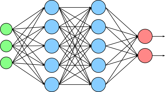
In this figure, the green nodes represent the input, the blue nodes represent the neurons of the two hidden layers, and the red nodes represent the neurons of the output layers. The arrows between nodes reflect the number of trainable weights of the network; we ignore the biases to keep the illustration simple.
Unstructured Pruning. In unstructured pruning, the goal is usually to introduce sparsity into the model by setting a certain percentage of the smallest-magnitude weights to $0$, assuming these have minimal influence on the model's output. Because it operates at such a fine-grained level, unstructured pruning can often achieve high compression ratios with little accuracy loss — especially when combined with retraining (or fine-tuning) to recover performance. We can visualize the setting of weights to $0$ by removing those weights from out architecture:
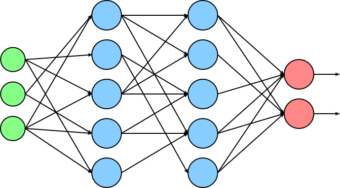
Setting a weight to $0$ only removes the value in case of sparse representations of weight matrices. However, most general-purpose hardware (like GPUs and TPUs) is optimized for dense matrix operations, not sparse ones. As a result, even if many weights are zeroed out, the model still requires dense memory storage and compute time unless custom sparse kernels or specialized hardware are used. In short, unstructured pruning does not inherently compress models in a hardware- or storage-efficient way, but it plays a critical role in analyzing model redundancy, reducing overfitting, and preparing models for more advanced compression pipelines.
Structured Pruning. In structured pruning, entire structures within a neural network — such as neurons, channels, filters, attention heads, or even whole layers — are removed, rather than just individual weights. The key idea is to eliminate coherent groups of parameters that contribute the least to model performance. The figure below illustrates this idea; notice how three neurons have been removed from the hidden layers of the original model as part of the pruning step.
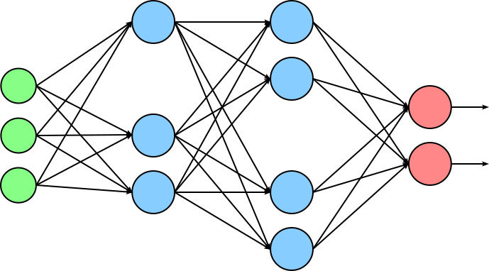
Structured pruning is especially valuable for achieving practical speedups and memory savings. Because the resulting model maintains a dense format with smaller dimensions — for example, the weight matrices of the two hidden layers in our pruned example network are now smaller — the model can be run efficiently on existing hardware like GPUs and TPUs without the need for sparse-specific optimizations. Structured pruning is often guided by importance metrics, such as the L1 or L2 norms of filters, attention scores, or sensitivity analyses. Once pruning is done, the model is usually fine-tuned to recover any accuracy lost due to the removal of structures. Structured pruning is widely used in real-world deployments of deep learning models, particularly in scenarios with strict latency or memory constraints (e.g., mobile devices, edge computing, or embedded systems). It offers a practical path to model compression that balances performance, simplicity, and hardware efficiency.
While structured pruning can lead to real improvements in speed and memory usage, it also has some downsides. One major challenge is that removing large parts of the model can hurt accuracy, especially if the pruned components were important. It can also be hard to tell which parts of the model are truly unnecessary, since common pruning methods often rely on rough estimates. Another issue is that pruning can create imbalances between layers, causing bottlenecks that limit performance. To avoid this, careful planning and retraining are usually needed, which adds extra time and cost. And even though structured pruning is more hardware-friendly than unstructured pruning, the actual speedups still depend on how well the pruned model fits the target hardware.
Quantization
The most common representation of trainable parameters during training is 32-bit floating-point (fp32) precision. This is because fp32 offers a high level of numerical precision and dynamic range, which is crucial for stable and accurate gradient calculations during backpropagation. Training deep neural networks involves many small and incremental updates to the weights, and fp32 helps ensure that these updates are not lost due to rounding or precision errors. Although mixed-precision training using formats like fp16 is becoming more popular — especially for speeding up training and reducing memory usage on compatible hardware fp32 is still widely used as the default in many frameworks because it provides more robust and reliable convergence, especially for complex models or tasks that are sensitive to numerical precision.
The issue is that fp32 requires $4$ bytes to store a single value, resulting in huge memory requirements in case of models with millions, billions, or even trillions of trainable parameters. To give some examples, the table below shows the number of trainable parameters and the required memory assuming fp32 precision (32 bits = 4 bytes per parameter) for some popular LLM architectures:
| Model | Parameters (approx.) | Memory @ fp32 (GB) |
|---|---|---|
| GPT-2 (large) | 774 million | ~3.1 GB |
| GPT-3 | 175 billion | ~700 GB |
| LLaMA 2 (7B) | 7 billion | ~28 GB |
| LLaMA 2 (13B) | 13 billion | ~52 GB |
| LLaMA 2 (70B) | 70 billion | ~280 GB |
| GPT-4 (est. 1T range) | 1 trillion (est.) | ~4,000 GB (4 TB) |
Note that the memory usage here is only for model weights in fp32. During training, additional memory is required for activations, gradients, optimizer states (e.g., Adam uses 3 times the weight size), so actual training memory can be 4-8 larger.
During inference, however, the neural network is no longer updating its parameters — it is simply using the learned weights and biases to compute outputs. This allows the use of reduced-precision formats (such as fp16, int8, or bfloat16) for the weights, biases and activations (i.e., intermediate outputs of neurons/layers), because small rounding errors introduced by lower precision generally do not significantly affect the final predictions. The model's structure and learned representations are typically robust enough to tolerate minor numerical approximations. For an every-day analogy, consider the following quote from a PyTorch blog post:
If someone asks you what time it is, you don’t respond "10:14:34:430705", but you might say "a quarter past 10".
This process of reducing the precision of trainable parameters and activations of (mostly) trained models for inferencing is called quantization. The general goal of quantization is to map high-precision values (e.g., fp32) to low-precision values of smaller range (e.g., int8). while preserving the overall distribution of values during the mapping.
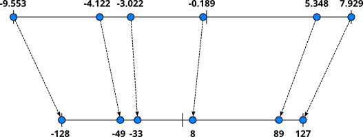
Apart from the chosen target precision, there are also various quantization strategies. One basic strategy is asymmetric quantization. In asymmetric quantization, we first find the minimum and maximum parameter value in a weight matrix. We then find a linear mapping $f(x)$ that maps the minimum and maximum parameter values to the range of the target precisions. For example, let's assume we want to quantize a weight matrix containing fp32 ($4$ bytes) values to int8 ($1$ byte) values; the range of int8 is $-128$ to $127$. Let's further assume that the minimum and maximum values in our fp32 weight matrix are $-9.533$ and $7.929$. Ignoring the details, it is relatively straightforward to find a linear mapping $f(x)$ such that $f(-9.533) = -128$ and $f(7.929) = 127$. We can then use $f(x)$ to convert all fp32 values in the weight matrix to int8 values. The figure below illustrates this idea.
Since we convert fp32 to int8 in our example, we can reduce the required memory by about 75%. The table below extends the previous table by including now the approximate memory requirements when representing the trainable parameters as int8 values.
| Model | Parameters (approx.) | Memory @ fp32 (GB) | Memory @ int8 (GB) |
|---|---|---|---|
| GPT-2 (large) | 774 million | ~3.1 GB | ~0.77 GB |
| GPT-3 | 175 billion | ~700 GB | ~175 GB |
| LLaMA 2 (7B) | 7 billion | ~28 GB | ~7 GB |
| LLaMA 2 (13B) | 13 billion | ~52 GB | ~13 GB |
| LLaMA 2 (70B) | 70 billion | ~280 GB | ~70 GB |
| GPT-4 (est. 1T range) | 1 trillion (est.) | ~4,000 GB (4 TB) | ~1,000 GB (1 TB) |
Again, these numbers refer only to the trainable parameters of the model — although those are the only ones that matter during inference. Keep in mind, however, that a full int8 quantization may not apply to all parts of the model (e.g., some layers might still use fp16/fp32), so real-world memory use can be slightly higher.
While basic asymmetric quantization and similar variants are relatively easy to implement in terms of finding and applying mapping $f(x)$, there are some practical challenges involved. One of the biggest problems are outliers, i.e., extreme values in the weight matrix. Since the minimum and maximum values in our weight matrix, outliers "artificially" increase the input range and negatively affect the definition of $f(x)$. To illustrate this, let's assume that the weight matrix from our previous example contains an outlier $-999.999$ as the new minimum. Using the same approach as before, we might get a mapping as illustrated by the figure below.
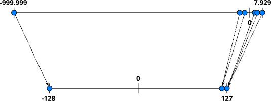
Particularly notice how now non-ouliers are mapped into a very small range in the target precisions, and many values are now more likely mapped to the same value, making them unable to distinguish any longer. These effects greatly increase the risk of performance degradation due to quantization. A basic counter-measures is clipping, where all fp32 weight values are cut to a minimum and maximum range. However, finding good cut-off values is not straightforward and typically requires some form of calibration. The main take-away message is that even basic strategies such as asymmetric quantization require careful considerations and implementations to minimize the degradation of performance of a quantized model.
On a high-level, quantization strategies come in three main flavors:
Post-Training Quantization (PTQ): In PTQ, the network is training using full precision (e.g., fp32) and the trainable parameters are converted to a lower-precision format (e.g., int8) after the model has been fully trained. As such, PTQ does not require retraining the model making It simpler and faster to implement, but may lead to slightly lower accuracy, especially in very sensitive models, compared to QAT.
Quantization-Aware Training (QAT): QAT simulates the effects of quantization (e.g., converting to int8) during the training process, rather than after training like in PTQ. The basic idea is to insert "fake" quantization operations into the computation graph that mimic the rounding, clamping, and precision loss of real quantization, allowing the model to learn to adapt to these constraints. During QAT, the model still uses fp32 weights and activations for backpropagation and gradient updates, but forward passes include simulated quantization effects. This helps the model adjust its parameters to reduce the accuracy loss that would otherwise occur due to quantization. As a result, QAT typically achieves higher accuracy than post-training quantization, especially in cases where the model is sensitive to precision loss.
Quantized Training (QT): QT (or integer-only training) is a more advanced form of quantization where both the forward and backward passes of training are performed using low-precision (e.g., int8) that will be used during inference. Unlike QAT, which simulates quantization effects but still uses float32 for gradients and weight updates, QT aims to train the entire model using quantized operations. However, this approach is much more challenging due to the difficulty of accurately computing gradients and performing updates with limited precision, and it often requires special techniques like custom optimizers, quantized gradient representations, and careful scaling strategies.
Overall, quantization is a useful approach to reduce the overall memory footprint of a model in a predictable manner. Quantization generally works best for (very) large models (incl. LLMs) as those models are more likely to be over-parameterized, and the reduced precision is likely to harm the model's performance. Still, quantization always involves some loss of information which may result in the degradation of the performance of a model. To help mitigate performance degradation, meaningful quantization strategies are required that take issues such as outliers into consideration.
Knowledge Distillation
Knowledge distillation (or model distillation) relies on the same observation as quantization — that is, the very large models are often over-parameterized and have more capacity than the complexity of the dataset or task requires. For example, foundation LLMs have billions and trillions of parameters, and have been trained over Web-scale datasets. Using such a general-purpose LLM to power, say, a domain-specific chatbot is often overkill. For such use cases — which are very common — a much smaller model with way less computational costs would often suffice.
The obvious alternative would be to train a smaller model and use mostly training data relevant to the target domain (e.g., a chatbot helping customers of a bank). However, training even a small(er) LLM from scratch is still very challenging and resource-intensive as the model not only has to learn the domain knowledge but also proper language, including the underlying complex patterns and subtle linguistic nuances, to generate well-formed sentences and paragraphs. On the other hand, we already have much larger foundation models that "know" language. So why not utilize this knowledge?
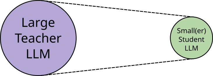
This is where knowledge distillation comes in. At its core, knowledge distillation, is about transferring knowledge from a large, complex "teacher" model (e.g., out pretrained foundation LLM) to a smaller, simpler "student" model; the figure below illustrates this overall idea. The teacher model is typically overparameterized and computationally expensive. The intuition is that the teacher model has learned a rich representation of the data (e.g., text and language). Instead of training the student model from scratch, it learns by mimicking output of the teacher model. This essentially guides the student model to learn a similar behavior as the teacher model but with much fewer trainable parameters.
There are various implementations of knowledge distillation to use a large teacher model for training a small(er) student model. Why implementation of knowledge distillation is applicable mainly depends on the available (domain-specific) training data, whether the trainable parameters of the teacher model are accessible (white box) or only the outputs of the teacher model can be used (black box), and the overall computational resources. Let's briefly go through some of the common approaches for knowledge distillation.
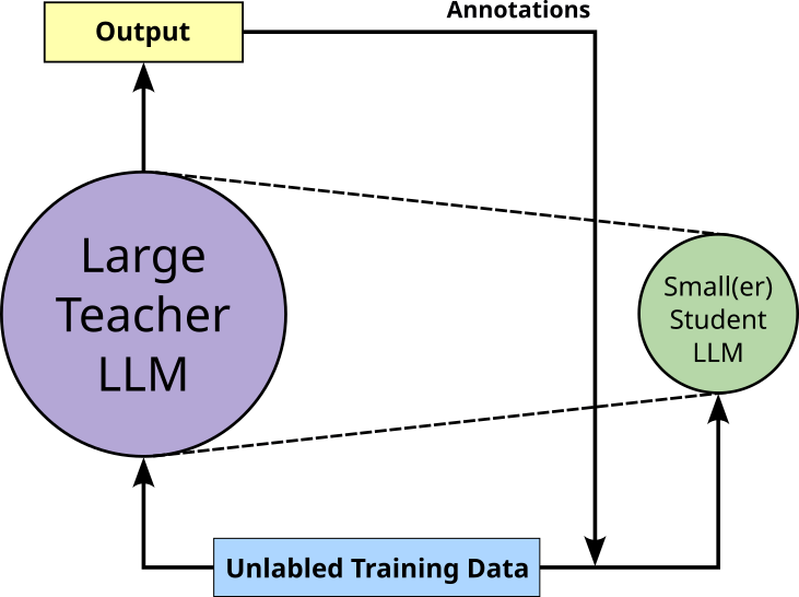
Response Distillation. The fundamental idea of response distillation is simply to use the teacher model to annotate an unlabeled dataset which is then used to train the student model; see the illustrations below. In other words, instead of manually annotating or creating the training dataset for the student model, we use the teacher model to "outsource" this task. For example, in case of the LLM, the unlabeled training data may consist of questions and the annotation provided by the teacher model are the corresponding answers.
Response distillation is very easy to implement, particularly if the teacher model is accessible via an API and, for example, there is no need to run a teacher LLM locally. This makes response distillation a black-box approach since no parameters or activations of the model are required. Assuming a good teacher model — which is the most fundamental assumption for knowledge distillation, the annotations provided by the teacher model are generally of high quality.
However, response distillation has its limitations and challenges. For one, creating annotations for large datasets needed to train the student model can be quite expensive, either in terms of compute or money (e.g., when using a paid API). Also, the final output of the teacher model does not capture more nuanced knowledge (compared to logits; see below) which often means the trained student tends to be less creative in terms of its responses to prompts. And lastly, response distillation requires that the teacher model was exposed to all relevant data during training to create correct annotations (e.g., answers to questions). This implies that we cannot use response distillation to train a very domain-specific model based on data not part of the training of the teacher model.
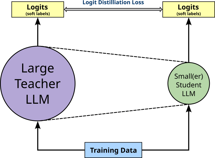
Logits Distillation. In case of logits distillation, both the teacher and student model receive the same input (e.g., a text prompt). Training the student model means to ensure that the output of the student model better and better mimics the output of the teacher model. As the name suggests, logits distillation considers the final logits as the outputs of both models. The reason is that the logits capture more information than the probabilities after the Softmax. Additionally, particularly in case of LLMs, it is much less straightforward to compute the similarity or the differences between the final text outputs. The logits of a model are generally considered internal values of a model, making logits distillation a black-box approach.
Logits distillation comes in two flavors. Logits distillation with teacher supervision only considers only the similarity or differences between the logits of both models. Training the student model here means minimize some logits distillation loss (e.g., KL Divergence) to make the student mimic the teacher; see the figure below.
As such, this form of logits distillation does not require an annotated dataset. Of course, this again means that the quality of the student model will highly depend on the quality of the teacher model. Without any ground truth, it generally makes it more challenging to properly evaluate the trained student model.
In contrast, if an annotated dataset containing ground truth is available, logits distillation with student loss can be implemented. Here both a distillation loss and the basic student loss — typically the cross-entropy loss between the predicted and ground truth labels — are minimized together to train the student. The figure below illustrates this extension to the overall setup.
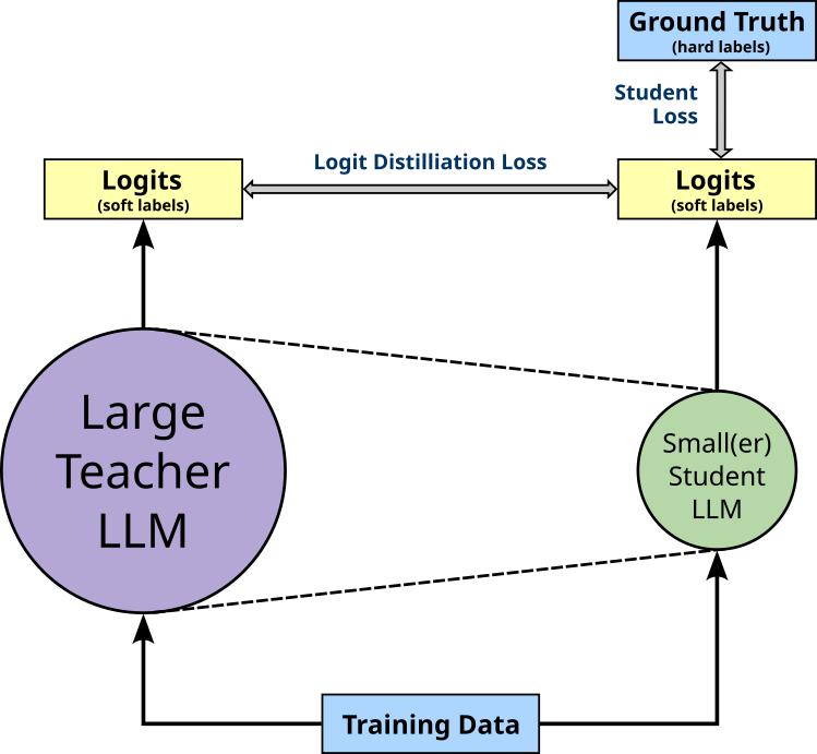
Including the basic student loss typically provides a richer training signal resulting in a more stable training, and allows for a straightforward evaluation using common metrics. Of course, considering both losses also adds complexity to the training. This includes that it is not obvious how both loss terms should be combined, and typically weight terms are used to balance between the importance of both losses. Lastly, there is the risk of conflicting signals when the output of the teacher model is very different than the ground truth. This can happen if the training data used for the distillation contains data completely unknown to the teacher model. Whether the output of the teacher model or the ground truth should be more trusted can be tweaked by the weight terms when combining both losses.
Feature Distillation. In feature distillation, the student model not only aims to mimic the teacher model with respect to the output, but also with respect to the internal representations (features or parameters). As such, feature distillation also minimizes the loss with respect to different activations (i.e., intermediate outputs) between both models; again, the figure below illustrates this idea on an abstract level. While not required, feature distillation is typically used in combination with logits distillation.
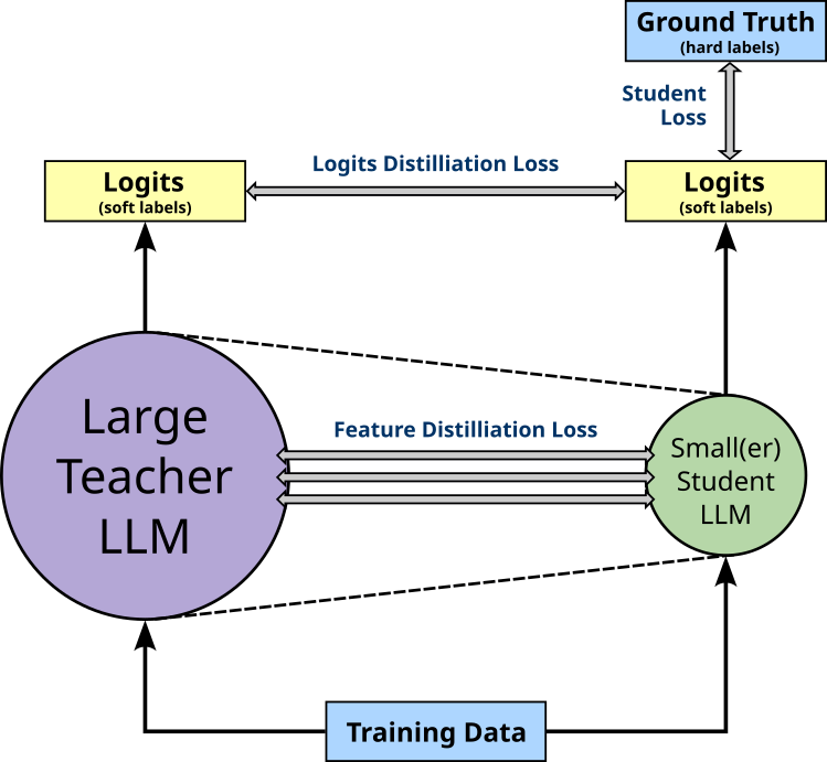
Intuitively, feature distillation provides an even richer signal compared to (just) logit distillation as it enables a "deeper" knowledge transfer beyond outputs. On the other hand, it further adds complexity to training of the student model via distillation. Since the student model is typically much smaller than the teacher model — for example, having fewer layers or fewer neurons per layer — it is not obvious how to align both models and to calculate the feature distillation loss. For example, a teacher LLM might have 32 Transformer layers while the student LLM only has 8 Transformer layers. Here, a common approach is to align each Transformer layer of the student with every fourth layer of the teacher. If the aligned layers then also have different sizes, additional strategies (e.g., learnable projects or feature pooling) are required to enable the meaningful computation of a loss.
Low-Rank Approximation
Another common compression method utilizing that most LLMs or other very large models are over-parameterized is low-rank low-rank approximation (or low-rank decomposition). The fundamental idea is to approximate a weight matrix $\mathbf{W}^{m\times n}$ with smaller low-rank matrices, say, $\mathbf{A}^{m\times r}$ and $\mathbf{B}^{r\times n}$ such that $\mathbf{W} \approx \mathbf{A}\mathbf{B}$. Naturally, to yield a meaningful compression, $r$ is chosen to be smaller than $m$ and $n$, i.e., $r < min(m, n)$. In short, the goal of the decomposition is is that the new number of weights (represented by matrices $\mathbf{A}$ and $\mathbf{B}$) is smaller than the initial number of weights in matrix $\mathbf{W}$ — without (significantly) affecting the overall performance of the model.
To better illustrate this idea, let's consider a simple linear layer containing $10$ neurons and expecting an input of size $10$. When implemented, this linear layer features a weight matrix $\mathbf{W}^{10\times 10}$ looking as follows:
This means that the weight matrix of this linear layer contains $100$ trainable parameters in total. Now let's assume we found two matrices $\mathbf{A}^{m\times r}$ and $\mathbf{B}^{r\times n}$ such that $\mathbf{W} \approx \mathbf{A}\mathbf{B}$, and let's assume $r = 3$ — that is, we now have two matrices $\mathbf{A}^{10\times 3}$ and $\mathbf{B}^{3\times 10}$ whose product approximates $\mathbf{W}$. Again, let's quickly visualize both matrices.
Both new weight matrices $\mathbf{A}$ and $\mathbf{B}$ now contain $30$ values each; thus, a total of $60$ trainable weights — compared to initial number of $100$ weights in $\mathbf{W}$. More generalized, weight matrix $\mathbf{W}$ contains $mn$ values, matrices $\mathbf{A}$ and $\mathbf{B}$ contain together $(mr+rn)$ or $r(m+n)$ values. We can therefore evaluate the memory requirements for the model after the decomposition using the following ratio:
Notice, that $r$ may need to be noticeably smaller than $m$ and $n$ to actually gain an advantage. For example, if we set $r=8$ in the use above, matrices $\mathbf{A}$ and $\mathbf{B}$ would contain $80$ weights each, resulting in $160$ weights altogether, which are obviously more than the initial $100$ weights in $\mathbf{W}$.
So far, we assumed that we were given the two matrices $\mathbf{A}$ and $\mathbf{B}$ such $\mathbf{AB}$ is a good approximation of the initial weight matrix $\mathbf{W}$. Of course, the challenge in practice is to actually find (i.e., compute) $\mathbf{A}$ and $\mathbf{B}$. The well-known task of matrix decomposition (also known as matrix factorization is the process of breaking a large matrix into a product of smaller, simpler matrices that capture the essential structure or properties of the original. This is often done to simplify computations, reveal hidden patterns, or enable efficient storage and processing. In practical terms, it allows complex operations — such as solving systems of linear equations, computing matrix inverses, or applying transformations — to be performed more efficiently by working with the decomposed components. Various algorithms for matrix decomposition exits, and which can be applied for low-rank approximation; here is just a brief outline of popular approaches:
Singular Value Decomposition (SVD): SVD is one of the most fundamental and widely used low-rank approximation methods. It is particularly effective for compressing large, fully connected layers. SVD decomposes a matrix $\mathbf{W}^{m\times n}$ into three matrices $\mathbf{U}^{m\times m}$, $\mathbf{S}^{m\times n}$, and $\mathbf{V}^\top$ such that $\mathbf{W} \approx \mathbf{U}\mathbf{S}\mathbf{V}^\top$. Matrix $\mathbf{S}$ is a diagonal matrix containing the singular values in descending order. The singular values represent the "strength" or importance of each dimension along which the original matrix acts. The compression happens by keeping only the top $k$ singular values (and their corresponding vectors in $\mathbf{U}$ and $\mathbf{V}^\top$), giving is $\mathbf{W} \approx \mathbf{U}_k\mathbf{S}_k\mathbf{V}_k^\top$. Using our inital terminology $\mathbf{A} = \mathbf{U}_k\mathbf{S}_k$ and $\mathbf{B} = \mathbf{V}_k^\top$. SVD is often applied to individual layers in a trained network (post-training compression).
Tensor Decompositions: While SVD is a matrix decomposition technique, many modern neural network components, such as convolutional layers and attention mechanisms in LLMs, are better represented as higher-order tensors. Tensor decompositions generalize SVD to these multi-dimensional arrays, and there are various algorithms. For example, Canonical Polyadic (CP) decomposition is particularly effective for convolutional layers. Tucker decomposition (or Higher-Order SVD) is a more flexible and general technique than CP decomposition. It often results in a better trade-off between compression and accuracy. It's been applied to both convolutional and fully connected layers.
Non-Negative Matrix Factorization (NMF): In contrast to SVD, NMF directly decomposes a matrix $\mathbf{W}$ into two smaller matrices $\mathbf{A}$ and $\mathbf{B}$ such that $\mathbf{W} \approx \mathbf{AB}$. However, as the name suggestions, NMF requires that all values in $\mathbf{W}$ are non-negative (i.e., $\geq 0$) — the resulting values in $\mathbf{A}$ and $\mathbf{B}$ will also be non-negative. This constraint regarding non-negativity poses challenges for model compression since the weights in a typical neural network, including LLMs, are not constrained to be non-negative. However, there are cases where NMF can be applied. For example, some layers naturally feature non-negative data (e.g., some embedding layers or attention matrices). Also some regularization strategies during training "encourage" non-negative weights.
There are also other, often more specialized, matrix decomposition techniques. However, more deeper exploration is beyond the scope of this notebook.
Side note: The most basic use case for low-rank approximation to reduce the memory footprint of a model is to take a pretrained model and replace a selected subset or all weight matrices with (hopefully good) approximations. This new and smaller model is then used for inferencing. However, the decomposition into smaller matrices is still perfectly differentiable and such could be used for training. For example, after applying SVD on a pretrained model, the compressed network can then additionally be fine-tuned to recover any lost accuracy. In fact, the concept of low-rank approximations has also become a very popular fine-tuning strategy, as we will cover later.
Efficient Pretraining
Pretraining refers to the initial phase of training a neural network model — especially LLMs — on a massive, general-purpose dataset before it is fine-tuned for specific tasks. During pretraining, the model learns broad patterns in language (e.g., grammar, syntax, semantics, world knowledge) by predicting missing tokens, next tokens, or masked tokens from text. This is typically done in a self-supervised manner, meaning the training data does not need human labeling. Once pretrained, the model can be fine-tuned on much smaller, task-specific datasets (e.g., for translation, question answering, or summarization) with relatively little additional training. This two-phase approach allows the model to generalize well across a wide range of tasks and domains.
Particularly pretraining large foundation LLMs is exceedingly time and resource-intensive. As such, any means to make the training more efficient can translate to significant cost savings. In the following, we outline some of the current approaches to reduce the memory footprint and/or speed up the training of a model. In practice, different strategies are often combined to improve the overall training efficiency.
Mixed Precision Training
The fundamental motivation behind mixed precision training is similar to idea of quantization (see above) — that is, the representation of the model's trainable parameters using a low(er)-precision representation to reduce the size of the model in terms of the required memory but also to speed up computations In case of basic quantization — which is primarily done to make a pretrained model more efficient for inferencing — we now want to work with lower precision as part for the actual training. The main difference here is the overall memory footprint is now determined by:
- Model weights (effectively the description of the model)
- Activations (intermediate values needed for backpropagation)
- Gradients (calculated during backpropagation)
- Optimizer states (e.g. for Adam: momentum and variance estimates)
Using quantization to reduce the size of the memory only concerns the model weights, but for training, all those aspects regarding memory consumption are important.
For training neural network models, we generally require a high precision to ensure a stable training since the gradients and parameter updates may involve very small values. However, fp64 (double precision) is generally not needed because it offers far more numerical precision and range than required. Neural networks are inherently robust to small numerical errors due to their approximate nature and stochastic optimization (like gradient descent). While fp64 can represent values with very high precision (about 15-17 decimal digits), this level of detail does not meaningfully improve training outcomes. On the other hand, fp16 (half precision) is often insufficient on its own due to its limited precision (~3-4 decimal digits) and narrow dynamic range. These constraints can cause issues like gradient underflow, where small values round down to zero, or overflow, where large values exceed representable limits — both of which can destabilize training. This is why fp32 has become the standard precision for training neural networks.
The idea of mixed precision training exploits the observation that performing some parts of the training fp16 precision does typically no harm a model's accuracy. In mixed precision training, key components of the model—such as weights, activations, and gradients — are stored and processed using fp16 to take advantage of its lower memory footprint and faster computation. However, because FP16 has limited precision and a smaller dynamic range, it can lead to instability or accuracy loss during training. To address this, a separate fp32 "master copy" of the model's weights is maintained. This FP32 copy is not used during the forward or backward passes but is crucial for accurate weight updates during the optimizer step, where it accumulates the gradients.
During each training iteration, a temporary fp16 version of the master weights is created and used for the forward and backward passes. This allows the training process to benefit from the reduced memory usage and faster throughput of FP16 computations. Meanwhile, the fp32 master ensures that numerical accuracy is preserved over time, especially during gradient accumulation and parameter updates. This hybrid strategy effectively reduces memory consumption and bandwidth demands while still maintaining training stability and final model accuracy. The figure below illustrates the overall training process using mixed precision. Notice that all calculations of the forward and backward pass (backpropgation) are down using fp16; only the actual update of the master weights are done using fp32.
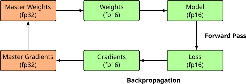
Since all the computations — forward and backward pass — are done using fp16, it may not be obvious why having the fp32 master copy of the weights is actually needed. This has two main reasons. For one, while fp16 is often sufficient to represent the gradients with sufficient precision, the gradients are first multiplied with the learning before performing the parameter updates. Since training LLMs commonly involve learning rates around $0.0001$ or $0.00005$, fp16 is often insufficient to appropriately represent the product. Secondly, in practice, a weight value is much larger than the weight update, adding both in fp16 can cause the update to effectively vanish. This happens because fp16 has limited precision (only 10 bits in the mantissa). If the weight is more than 2048 times larger than the update, the update gets right-shifted too much during addition, possibly to the point where it becomes zero. To avoid this, updates are typically computed and accumulated in fp32, which has much higher precision and range.
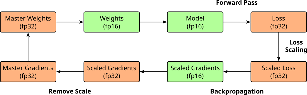
Although fp16 is often sufficient to store the gradients (i.e., before the multiplication with the learning rate), the gradients can become very small so that they will underflow and be treated as zero. This means no meaningful update happens for the affected parameters. The common approach to address this issue is called loss scaling. In loss scaling, the loss value is first multiplied by a scaling factor — often using a constant factor such as 128 or 1024 — before backpropagation begins. This boosts the magnitude of the resulting gradients, helping ensure they stay within the representable range of FP16 and do not underflow to zero. After the gradients are computed, the same scaling factor is divided out just before the optimizer step, ensuring that the final weight updates remain mathematically correct. The figure below shows the extended process of mixed precision training with loss scaling.
Mixed precision training has been shown to significantly improve training performance for large models, including large language models (LLMs), by reducing memory usage and increasing computational throughput. By performing most operations in FP16 while maintaining critical values like weight updates in fp32, it enables faster training on modern hardware — particularly GPUs with specialized support for half-precision arithmetic. Despite the reduced precision, mixed precision training achieves comparable accuracy to full fp32 training in practice. Techniques like loss scaling help preserve numerical stability, ensuring that model quality is not compromised. As a result, mixed precision has become a standard approach for efficiently training state-of-the-art neural networks at scale.
Scaling Models
The idea of scaling large models such as LLMs from smaller models is to train progressively larger architectures by leveraging insights, weights, or design patterns learned from smaller versions. Instead of starting from scratch with a massive model, researchers often begin with a smaller, computationally cheaper model to experiment with hyperparameters, architectures, optimization strategies, and training data. Once these settings are tuned, the same or similar configurations are applied to progressively larger models. This strategy is particularly valuable for LLMs because training from scratch at extreme scale is expensive and risky. Starting small allows researchers to identify bottlenecks like gradient instability or underfitting before committing millions of GPU-hours. It also provides a smoother pathway to frontier-scale performance while controlling costs and avoiding catastrophic training failures that would be far more costly with a massive model.
"Reverse" Model Compression Strategies.
We saw that model compression aims to convert a complex model into a smaller and/or simpler one to reduce the memory footprint and speed up inference time, without sacrificing the model's accuracy (too much). Some of these strategies can be "flipped" and used to scale up smaller/simpler models into more complex models with more capacity.
Low-Rank Approximation. If we assume that $\mathbf{W}^{m\times n}$ will be some weight matrix in our final model, we can first replace $\mathbf{W}$ with the product $\mathbf{AB}$ of two smaller matrices $\mathbf{A}^{m\times r}$ and $\mathbf{B}^{r\times n}$ — with $r$ being (much) smaller than $m$ and $n$ — during the early stage of the training. Then, we reconstruct $\mathbf{W}$ by calculating $\mathbf{W} = \mathbf{AB}$ and continue training using the full matrix $\mathbf{W}$. The assumption again is that the low-rank approximation of $\mathbf{W}$ — which is faster to train since the number of weights is much smaller — will be very close to the final matrix $\mathbf{W}$, so only little late-stage training with the full matrix is needed.
Knowledge Inheritance. The idea of knowledge inheritance is similar to knowledge distillation (see above), but with the difference that the smaller pretrained model acts as the teacher, and the student is the new, larger model we want to train. Since we assume that the student model will at some point surpass the accuracy of the teacher model, the impact of the teacher model needs to decrease during training — for example, but decreasing the weight of the logits distillation loss over time.
Model Growth for Progressive Training.
The basic idea behind using model growth for progressive training is to build and train a large neural network incrementally. Instead of training a massive model from scratch, you begin with a smaller, more manageable network. Once this smaller network is sufficiently trained, you expand it by adding new layers or modules (more depth), or by increasing layers (more width). The weights from the smaller, pretrained model are used to initialize the corresponding layers in the new, larger network. By starting small, you can use less computational power and memory, and the training process is more stable. The pretrained weights from the smaller model act as an excellent starting point for the larger one, helping to avoid the problematic "cold start" of randomly initialized weights. This process is repeated, gradually increasing the model's size and complexity, with each new iteration benefiting from the knowledge learned in the previous, smaller stage — hence, progressive training.
Basically all popular modern LLMs rely on the Transformer architecture. As quick recap, the main parameters of the Transformer architecture the determine the size of a model in terms of its required memory — and with that also the required training — are:
- Number of layers $n_{layers}$: the number of Transformer blocks or encoder/decoder layers
- Number of attention heads $n_{heads}$: the number of attention heads in each multi-head attention layer
- Hidden size or model dimension $d_{model}$: the size of the embedding vectors and the main hidden representation in the model
- Feed-forward network (FFN) dimension $d_{ffn}$: the size of the intermediate layer in the position-wise feed-forward network
To give some examples, the table below shows the values for the popular models of the GPT family. Note that at the time of writing, OpenAI has not released the numbers for its more recent and larger models. Still the main take-away message is that more complex and thus more capable models are essentially just scaled-up versions of simpler models (ignoring changes to the training data).
| Model | $n_{layers}$ | $n_{heads}$ | $d_{model}$ | $d_{\text{\textit{ffn}}}$ |
|---|---|---|---|---|
| GPT-1 | 12 | 12 | 768 | 3,072 |
| GPT-2 Small | 12 | 12 | 768 | 3,072 |
| GPT-2 Medium | 24 | 16 | 1024 | 4,096 |
| GPT-2 Large | 36 | 20 | 1280 | 5,120 |
| GPT-2 XL | 48 | 25 | 1600 | 6,400 |
| GPT-3 125M (Ada) | 12 | 12 | 768 | 3,072 |
| GPT-3 350M (Babbage) | 24 | 16 | 1024 | 4,096 |
| GPT-3 760M (Curie) | 24 | 16 | 1536 | 6,144 |
| GPT-3 1.3B (Babbage-002) | 24 | 24 | 2048 | 8,192 |
| GPT-3 2.7B | 32 | 32 | 2560 | 10,240 |
| GPT-3 6.7B | 32 | 32 | 4096 | 16,384 |
| GPT-3 13B | 40 | 40 | 5120 | 20,480 |
| GPT-3 175B (Davinci) | 96 | 96 | 12288 | 49,152 |
A wider range of strategies have been proposed to take a small(er) pretrained model and scale it up by increasing any subset of $n_{layers}$, $n_{heads}$, and $d_{model}$, $d_{\text{\textit{ffn}}}$ and use the available weights from pretrained model to kick-start the training of the now larger model in smart way. Just give one example for the Transformer architecture here, an approach proposed early on is to increase the number of layers $n_{layers}$ and simply copy over the weights from lower layers — also called stacking. This approach relies on the observation that the weights across all layers in a pretrained model often show a similar distribution. Thus, the weights of a lower layer make a good initialization of a higher layer. The figure below illustrates the idea of stacking using a Transformer encoder for a BERT model.
In this example, we start with a small pretrained model containing 3 encoder layers. We then create the larger model by duplicating the 3 encoder layers to now have 6 encoder layers in total. The red arrows indicate the weights from which the pretrained layer get copied to the newly added layer; of course, the weights of the embedding and classifier layer get also directly copied over. The larger model is then trained as a whole which includes updates of all weights across all layers. After the training, this process can be repeated by again duplicating the encoder layers, copying over the weights, and training the new model. The assumption/expectation is that the copied weights serves as a good initialization of the newly added layers to speed up the training process of the scaled model.
Various strategies for model growth in progressive training exist, aiming to build large, high-performing models by starting with smaller, more manageable ones and gradually expanding their capacity. Beyond adding more layers as shown in the example, other common approaches include widening existing layers, increasing the number of attention heads, or expanding hidden dimensions over time. Some methods also involve progressively growing the vocabulary or embedding sizes, or gradually unfreezing parameters that were initially fixed. However, most model growth strategies rely on specific assumptions and require careful design to work effectively. For instance, they often assume that the knowledge learned in the smaller model will transfer well to the expanded architecture without significant degradation, and that the optimizer and learning rate schedule can handle the sudden increase in parameters. Decisions such as when and how to grow the model, how to initialize new parameters, and how to avoid catastrophic forgetting or instability are crucial. Without careful consideration of these factors, progressive training can lead to inefficient scaling, unstable convergence, or suboptimal performance compared to training the full model from scratch.
Initialization Techniques
Weight initialization plays a critical role in the training of neural networks, especially large models such as LLMs, because it directly affects how signals propagate through the network during both the forward and backward passes. If the initial weights are too small, activations can vanish as they pass through many layers, leading to very small gradients and slow or stalled learning (vanishing gradients). Conversely, if the weights are too large, activations and gradients can explode, causing instability and divergence during training. Proper initialization helps maintain a stable variance of activations and gradients across layers, ensuring that the learning signal remains strong from the input to the output and back again. For large language models, the sheer depth and parameter count amplify any issues caused by poor initialization. In such architectures, small imbalances in early layers can compound exponentially, leading to numerical instability, gradient collapse, or even complete training failure.
For very large architectures like LLMs, initialization strategies are chosen with extreme care to keep activations and gradients stable across hundreds of layers and billions of parameters. Some common approaches include:
Xavier / Glorot Initialization is designed for $\text{tanh}$ or $\text{sigmoid}$ activations, Xavier initialization scales weights based on the number of input and output units ($\text{\textit{fan}}_{in}$ and $\text{\textit{fan}}_{out}$) so that the variance of activations is preserved. While it’s less common for modern transformers that use ReLU or GELU, it remains a foundation for understanding scaling principles.
Kaiming (He) Initialization is optimized for ReLU-type activations, this method scales by $\sqrt{2/\text{\textit{fan}}_{in}}$ to prevent the shrinking of signal variance as it moves forward. Some transformer feed-forward layers use a Kaiming-like initialization to match their activation functions.
Normalized Initialization with Dimension-Based Scaling: In transformers, weights (especially in attention projections) are often initialized from a normal distribution with variance inversely proportional to the hidden dimension. For example, attention logits are scaled by $1/d_k$ — where $d_k$ is the hidden dimension of an attention head — to prevent large values that could saturate the softmax, and some initializations multiply weight standard deviation by $1/n_{layers}$ to avoid residual stream blow-up in deep stacks.
DeepNorm / μParam Scaling: Newer LLM training strategies modify initialization together with residual connection scaling to keep both forward activations and backward gradients stable in very deep networks. For example, DeepNorm scales residual branches by constants like $\alpha = (2N)^{0.25}$, where $N$ is the number of layers. μParam scaling adjusts weight initialization so model capacity grows without destabilizing gradient magnitudes.
In practice, LLM training often combines these methods—using variance-preserving Gaussian initializations with careful per-layer scaling, orthogonal setups for stability, and explicit normalization (LayerNorm or RMSNorm) to continually re-stabilize the signal throughout the network. Without these refinements, models like GPT or PaLM could suffer severe instability long before convergence.
Training Optimizers
Optimizers are algorithms that adjust the parameters (weights and biases) of a neural network during training to minimize a loss function. They determine how the model learns from the data by deciding the size and direction of each parameter update based on the computed gradients from backpropagation. The optimizer's role is crucial because the way it navigates the high-dimensional loss landscape directly affects training speed, stability, and the final model quality. The purpose of an optimizer is to find parameter values that produce accurate predictions while using computational and memory resources efficiently.
Basic optimizers like Stochastic Gradient Descent (SGD) update parameters using the raw gradient information, while more advanced ones — such as Adam, AdamW, Adafactor, and Lion — adapt the learning rate for each parameter based on historical gradient information. This adaptation helps deal with challenges like noisy gradients, ill-conditioned optimization surfaces, and varying gradient magnitudes across layers. In large models such as LLMs, optimizers must also address scale-related challenges: keeping training numerically stable across billions of parameters, reducing the risk of exploding or vanishing gradients, and managing memory overhead. The following table lists some popular optimizer algorithms and their (potential) limitations for training LLMs.
| Optimizer | Why It's Used | Limitations for LLMs |
|---|---|---|
| SGD (with or without momentum) | Simple, memory-efficient, and reliable for well-conditioned problems. Works well when combined with momentum and learning rate schedules. | Converges slowly in high-dimensional, non-convex spaces; very sensitive to learning rate choice; requires more tuning and warmup. |
| Adam / AdamW | Adaptive learning rates per parameter; fast convergence; robust to gradient scaling. AdamW decouples weight decay from momentum. | 2-3x memory usage due to first and second moment states; hyperparameter sensitivity; can still diverge without proper init/normalization. |
| Adafactor | Memory-efficient alternative to Adam (factorized second-moment storage); used in T5 and other huge models. | Less stable in small-batch or fine-tuning; needs careful learning rate warmup and gradient clipping. |
| Lion (Evolved Sign Momentum) | Lower memory than Adam (stores only momentum); competitive performance on LLMs; efficient update rule. | Relatively new; limited large-scale production use; hyperparameter tuning can be sensitive. |
In short, common optimizers trade off memory requirements with stability when it comes to training very large networks. Training LLMs efficiently requires specialized optimizers because their massive scale — often billions or trillions of parameters — pushes standard methods to their limits. Common algorithms like vanilla SGD may converge too slowly in such high-dimensional spaces, while adaptive methods like Adam triple memory usage due to extra parameter states. At this scale, inefficiencies in computation or communication quickly multiply, making training both costly and slow. Beyond memory concerns, large models have highly varied gradient magnitudes across layers, and without adaptive scaling, training can become unstable or diverge. Deep architectures like transformers also introduce risks such as exploding attention scores and residual growth, demanding optimizers that work hand-in-hand with careful initialization, normalization, and mixed-precision stability.
System-Level Pretraining Efficiency Optimization
In simple terms, training a neural network comes down to performing many matrix and vector operations. This means that almost all the computations involved — both in the forward pass (making predictions) and the backward pass (computing gradients) — can be expressed as linear algebra. Inputs, weights, and activations are represented as vectors and matrices, and the core operations are matrix multiplications, additions, and element-wise functions. For example, in each layer, the network computes $\mathbf{y} = \mathbf{W}\mathbf{x} + \mathbf{b}$ to transform the data, and during backpropagation it uses similar matrix operations to calculate weight updates.
This mathematical structure is why hardware like GPUs, which excel at parallel linear algebra, can train neural networks so efficiently. GPUs contain thousands of cores designed to execute these operations in parallel, significantly speeding up training compared to CPUs, which have far fewer cores optimized for sequential processing. This parallelism allows GPUs to process large batches of data and compute gradients for many parameters at once, reducing training time from weeks to days or even hours. For very large models such as LLMs, the sheer scale of parameters and computations makes GPU acceleration not just advantageous but practically mandatory. These models can have hundreds of billions of parameters, requiring enormous memory bandwidth and compute throughput to train efficiently.
LLMs and other networks have become so large that training them on a single GPU — that is, a single piece of hardware containing all cores and memory — is no longer feasible but requires large computing clusters with multi-GPU setups. Training LLMs on large GPU clusters introduces challenges in communication, synchronization, and workload distribution. This requires frequent exchange of large amounts of data — such as gradients, parameters, or activations — between GPUs, often across different machines. Even with high-speed interconnects like NVLink or InfiniBand, communication overhead can become a bottleneck, reducing the theoretical scaling efficiency. Synchronization delays also arise because all GPUs must stay in step during training; if one GPU is slower (e.g., due to uneven workload), it can stall the entire system. Another challenge is fault tolerance and system stability at scale. Large clusters have thousands of GPUs running for days or weeks, so hardware failures, network issues, and software bugs are inevitable. Memory management is also a concern—storing massive models, optimizer states, and activation buffers requires careful sharding and offloading to prevent GPU memory overflow.
Efficiently training LLMs in GPU clusters relies on a combination of parallelization strategies, memory optimizations, and advanced scheduling techniques to maximize throughput while minimizing communication overhead. The most common strategies include data parallelism (replicating the model across GPUs and splitting the training data), tensor/model parallelism (splitting large layers across GPUs so that each GPU handles part of the computation), and pipeline parallelism (breaking the model into stages that process different microbatches in sequence). Frameworks like Megatron-LM and DeepSpeed often combine these into 3D parallelism, which integrates all three to scale across thousands of GPUs.
Advanced methods focus on reducing the communication and memory costs of these strategies. ZeRO (Zero Redundancy Optimizer) partitions optimizer states, gradients, and parameters across devices to avoid storing full copies on each GPU. Activation checkpointing trades extra computation for lower memory usage by recomputing activations instead of storing them. Mixed precision training (see above) speeds up computation and reduces memory footprint without significant accuracy loss. More recent approaches include sequence parallelism (splitting sequences across GPUs for long-context models), gradient compression (quantizing or sparsifying gradients before communication), and asynchronous communication to hide latency. Together, these methods allow LLM training to scale to hundreds of billions of parameters without being bottlenecked by GPU memory or interconnect bandwidth.
Efficient Fine-Tuning
The purpose of fine-tuning large pretrained LLMs is to adapt their broad, general knowledge to perform well on a specific task, domain, or style. While pretraining equips the model with strong language understanding and general knowledge, it does not guarantee optimal performance in specialized contexts — such as legal analysis, medical text processing, or technical customer support. Fine-tuning refines the model's responses using targeted data so it can use domain-specific terminology correctly, follow specialized reasoning patterns, and align with desired output formats or tones. Fine-tuning is needed because training a large model from scratch is prohibitively expensive in terms of data, computation, and engineering effort. By leveraging the general-purpose abilities gained during pretraining, fine-tuning can achieve high accuracy and domain relevance with far less cost and data. It also ensures that models remain up to date with evolving knowledge, regulations, or user needs, making them more reliable and useful in real-world applications.
However, fine-tuning LLMs also comes with several challenges, both technical and practical. A key issue is catastrophic forgetting, where the model loses some of its general capabilities or pretraining knowledge when overfitted to the fine-tuning dataset. This can make the model perform worse on tasks outside the fine-tuned domain. Closely related is overfitting, which occurs when the fine-tuning data is too small or too narrow, leading the model to memorize rather than generalize — producing brittle, biased, or repetitive responses. More generally, specialization with general usefulness is non-trivial: too much fine-tuning can narrow the model’s capabilities, while too little may fail to achieve the desired performance improvements. Lastly, fine-tuning large models still requires substantial computational resources — even if it is far cheaper than training from scratch, the process still demands powerful GPUs, careful hyperparameter tuning, and memory-efficient techniques to handle billions of parameters.
Parameter-Efficient Fine-Tuning
Parameter-efficient fine-tuning (PEFT) is an approach to adapting large pretrained models, such as LLMs, by updating only a small subset of their parameters instead of all of them. Traditional fine-tuning requires modifying every parameter in the model, which is computationally expensive and storage-heavy, especially for models with billions of parameters. PEFT methods, like LoRA (Low-Rank Adaptation), adapters, or prefix-tuning, inject small trainable modules into the network or adjust low-rank projections, allowing the core pretrained weights to remain frozen. This significantly reduces the number of trainable parameters while still achieving strong task-specific performance. PEFT has two key advantages:
Efficiency: Fine-tuning a full LLM can require hundreds of gigabytes of GPU memory, long training times, and high storage costs for each specialized version of the model. In contrast, PEFT methods require far fewer resources, making it feasible to train and store many domain-specific adaptations from a single base model. This is especially valuable when an organization needs multiple specialized variants without duplicating the entire LLM for each case.
Flexibility and maintainability:. Since PEFT keeps the base model intact, it is easy to swap in or combine different fine-tuned modules, update them independently, or revert to the original general-purpose model when needed. This modularity also enables faster experimentation and safer deployment, as the risk of degrading the base model's broad capabilities is minimized (e.g., catastrophic forgetting).
The core assumption behind PEFT is again that large models such as LLMs are often over-parameterized and that the changes needed to adapt such a model to a new task often lie in a low-dimensional subspace. By only training a small/reduced set of parameters, PEFT strategies often achieve nearly the same performance as full fine-tuning while requiring far less memory, computation, and storage. In short, PEFT makes fine-tuning large models practical, cost-effective, and scalable while retaining most of the performance benefits of full fine-tuning. Let's go over some of the common approaches for parameter-efficient fine-tuning.
Low-Rank Adaption (LoRA)
As the name suggests, LoRA is closely related to low-rank approximation of model compression. LoRA adapts large pretrained models by adding small, trainable low-rank matrices to certain weight matrices &mdashl; typically in the attention and feed-forward layers — while keeping the original weights frozen. Instead of updating the full weight matrix $\mathbf{W}^{m\times n}$ (which can be very large), LoRA learns two much smaller matrices $\mathbf{A}^{m\times r}$ and $\mathbf{B}^{r\times n}$ whose product approximates the necessary update $\Delta \mathbf{W} = \mathbf{AB}$, which then yields the final output of the layer $\mathbf{h} = \mathbf{W} + \Delta\mathbf{W}$. The matrices $\mathbf{A}$ and $\mathbf{B}$ have dimensions chosen so that the rank $r$ is much smaller than the original matrix size, drastically reducing the number of trainable parameters. The figure below illustrates the idea of LoRA.
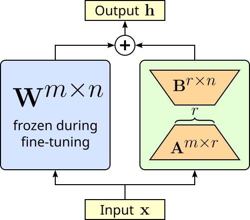
Matrix $\mathbf{A}$ is typically initialized with some random Gaussian noise,i.e., $\mathbf{A} \sim \mathcal{N}(0, \sigma^2)$), while matrix $\mathbf{B}$ is initialized with all elements being $0$, i.e., $\mathbf{B} = 0$. This means that at the beginning of the fine-tuning $\Delta\mathbf{W} = 0$ so that the output of the layer is only determined by the original weight matrix $\mathbf{W}$. Of course, during the fine-tuning, matrices $\mathbf{A}$ and $\mathbf{B}$ will get updated during backpropagation so that $\Delta\mathbf{W} \neq 0$.
Adapter-based Tuning
In general, adapters are small, trainable neural network modules inserted into the layers of a large pretrained model to enable task-specific adaptation without modifying the original model's parameters. During fine-tuning, only the adapter parameters are updated, while the vast majority of the model's weights remain frozen. Typically, an adapter is a bottleneck layer that projects the high-dimensional hidden states of the model down to a smaller dimension, applies a nonlinearity, and then projects them back up to the original dimension before passing them to the next layer. This allows the adapter to learn compact task-specific transformations while keeping the base model intact. The figure below shows a simple adapter in the form of a bottleneck layer.
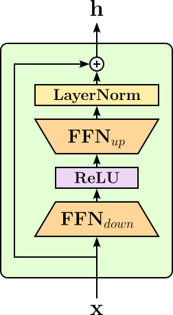
Here, the first fully connected network (FFN) layer maps the input down into a lower-dimensional representation. After applying a non-linear activation function, a second FFN layer maps the activation back up into the same dimension of the input. The example above also performs layer normalization (LN) at the end — while the adapters can be arbitrarily complex, simple modules as shown here are very common. Adapters also have a residual connection so they can adjust the pretrained model's representations without overwriting them, preserving the general knowledge learned during pretraining while adding small, task-specific refinements. This design also helps with stable training as the output starts as identical to the pretrained hidden state, the fine-tuning process can gradually incorporate task-specific modifications instead of making abrupt changes to the model's internal representations.
Adapters can then be inserted into a pretrained model parallel to existing layers, sequentially (i.e., between existing layers), or both (hybrid). The following figure illustrates the basic setup for all three alternatives.
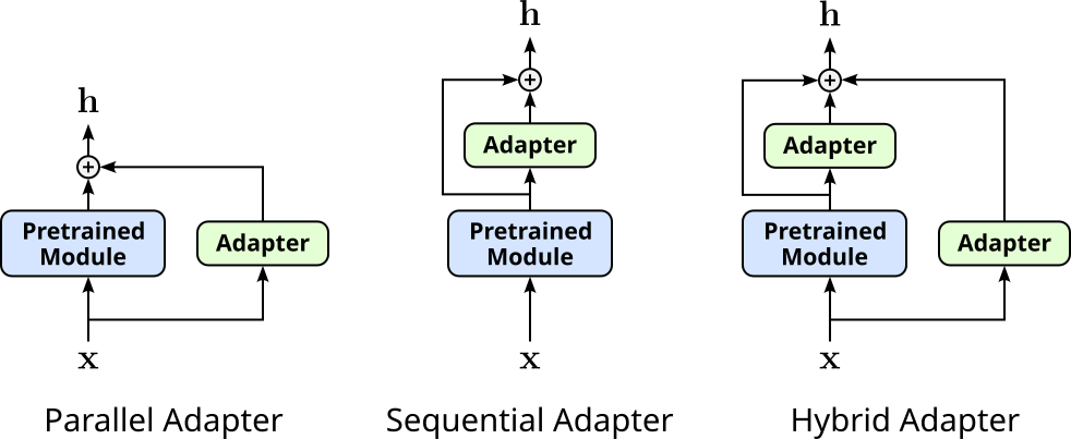
You may notice that parallel adapters are very similar to LoRA, and in some sense they are closely related. However, adapters are complete modules (i.e., small sub networks with linear layers, activation functions, normalization layers, etc.) and are inserted parallel to complete modules of the pretrained model. In contrast, LoRA "only" inserts low-rank approximations parallel to a single weight matrix, typically of a single linear layer.
Prompt Tuning
Although LLMs (e.g., GPT, LLaMA) are trained to "simply" predict the next token given a current sequence of tokens, both the training datasets and the models' capacities are so large that the models shows emergent capabilities — that is, LLMs can perform tasks they have not been explicitly trained for. Training on massive text corpora to predict the next token forces the model to learn deep patterns about language, knowledge, facts, reasoning chains, and even some world understanding, all embedded implicitly in the data. Even without explicit supervised task labels — such as input-target pairs for machine translation, question-answer pairs — the model sees tons of diverse text during training, including, for example:
- Translations embedded in parallel corpora or multilingual texts.
- Instructions and question-answer pairs.
- Code snippets, stories, dialogues.
This is why, with the "right prompt", we can ask a pretrained LLM to, say, translate a sentence from English to German. However, there are arbitrary ways to prompt the LLM and not all ways may yield satisfactory results. For example, here are some very basic prompts we might use to get the translation of an English sentence:
- "Translate English to German: Hello, how are you?"
- "English: Hello, how are you? German:"
- "Translate this to German: Hello, how are you?"
- "What is 'Hello, how are you?' in German?"
While for humans the intention of all four alternatives is clearly the same, it is not obvious if this is also true for the LLM, or if one alternative might perform better than the others. The questions is therefore: For a given task — here: English-to-German translation — can we learn the best prompt. Of course, tokens themselves are discrete values and backpropagation requires gradients, which are continuous and differentiable signals used to update parameters. However, recall that the first step of an LLM is to convert tokens into continuous embedding vectors, which can be learned via backpropagation. And this is where prompt tuning comes into play.
After converting an user prompt into its corresponding sequence of embedding vectors, prompt tuning prepends a fixed number of additional embedding vectors to this sequence. At the beginning (before the training), these additional embedding vectors are randomly initialized. This final sequence of vectors is then given to the pretrained LLM during training. The important detail is that after backpropagation only the additional embedding vectors are updated — all parameters of the pretrained LLM (incl. in the embedding layer) remain unchanged. The figure below illustrates this idea assuming a encoder-decoder LLM fine-tuned for an English-to-German machine translation task assuming "Translate English to German: Hello, how are you?" as input prompt (and "Wie geht es dir?" being the German translation).
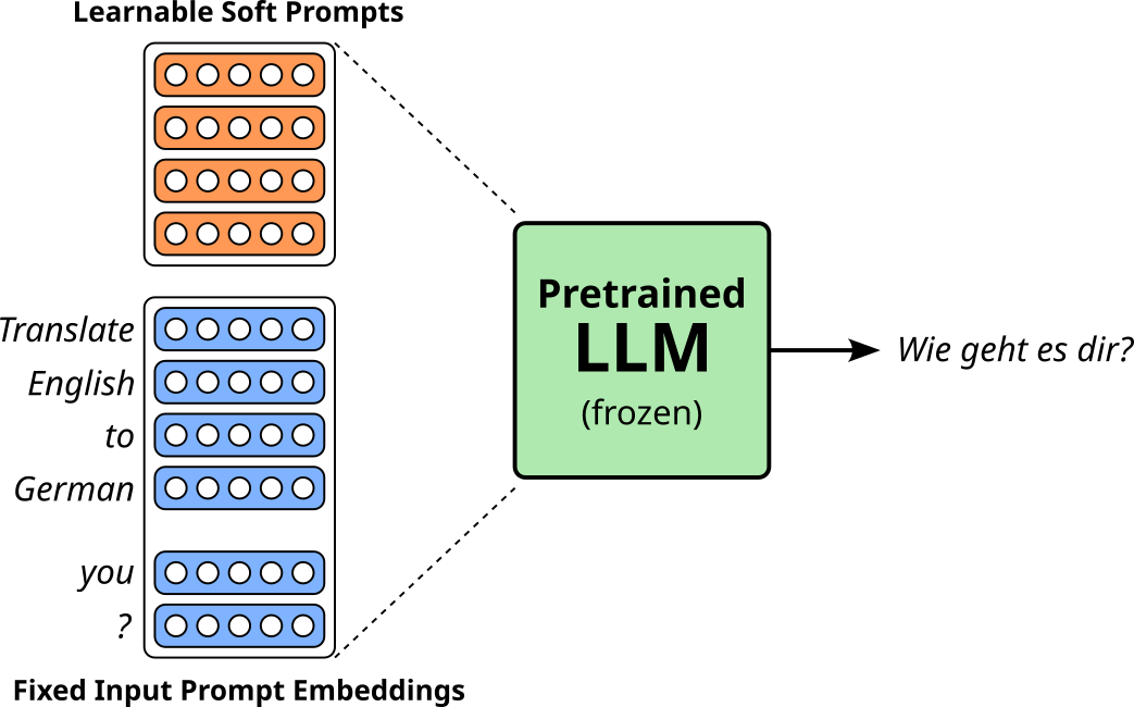
In this example, to keep it simple, we only add 4 embedding vectors to the initial sequence of vectors from the pretrained embedding layer; and only those 4 vectors are getting updated during training. Since these additional vectors are treated by the LLM as additional words/tokens, but do not represent actual words/tokens, these added embedding vectors are also called soft prompts (compared to actual text prompts considered hard prompts) — you could find the tokens in your vocabulary with embedding vectors closest to the soft prompt vectors, but there is no expectation that the tokens are in any way meaningful.
The obvious advantage of prompt tuning is, of course, the number of parameters that we train is very small. All parameters (weights, biases, etc.) of pretrained LMM are frozen and do not get updated after backpropagation. This also means that prompt tuning does not negatively affect the overall capabilities of the LLM to generate well-formed text. Another benefit is modularity since different soft prompts can be swapped in and out for different tasks without retraining the model itself. For example, besides our learned soft prompt for English-to-German machine translation, we might also have learned soft prompts for sentiment analysis, document summarization, or question answering.
However, prompt tuning also has limitations. Since it does not alter the internal weights of the model, it relies entirely on the model's existing knowledge and representational space. In simple terms, this means that the pretrained model is already capable of solving the specific tasks, but benefits from the additional "guidance" provided by the learned soft prompts. Thus, the model may underperform compared to full fine-tuning on tasks that require significant adaptation or domain-specific knowledge the model has not already learned. This also implies that soft tuning often works best for very large models; smaller models may not benefit as much because their representations are less rich and flexible. Prompt tuning can also be sensitive to the initialization of the soft prompts, and in low-resource settings, it may converge more slowly or get stuck in suboptimal solutions.
Prefix Tuning
Prefix tuning is very similar to the idea of prompt tuning. Both methods adapt a large pretrained language model by learning a small set of task-specific continuous vectors (i.e., the soft prompts) while keeping the model's original weights frozen. The main difference is where these soft prompts are inserted. In prompt tuning, the learned vectors are prepended to the input embeddings only once before the first Transformer layer. They act like extra tokens that influence the model’s behavior through all subsequent layers, but no additional parameters are added deeper in the network.
In prefix tuning, the idea goes further: instead of adding the soft prompts only at the input, a learned "prefix" is injected into the key and value matrices of the self-attention mechanism in every transformer layer. This means that at each layer, the model can attend to both the real sequence tokens and the layer-specific prefix vectors. Each layer has its own prefix parameters, allowing for more fine-grained control over the model's internal attention patterns. The figure below illustrates this idea by showing the basic architecture of the original Transformer layer together with the injected prefixes $\mathbf{P}_K$ and $\mathbf{P}_V$ to the key matrix $\mathbf{K}$ and the value matrix $\mathbf{V}$, respectively (here for the self-attention block).
Another difference compared to prompt tuning is that the prefixes are typically not directly soft prompts, i.e., a small fixed number of learnable vectors. It has been empirically shown that the direct use of soft prompts as prefixes often results in unstable training. In practice, the prefixes are therefore commonly learned by feeding the soft prompts into a small additional network that gets also updated during training. This step is also called reparameterization. For example, we assume a simple 2-layer fully connected network (FNN) layer, we get the prefixes $\mathbf{P}_K$ and $\mathbf{P}_V$ as follows:
where ${E}_{SP}$ is the embedding matrix containing a fixed number of soft prompts. Of course, here we assume that the $FFN$ module is designed such that the output dimensions of the prefixes match the dimensions of the key and value matrices for easy concatenation. Note that after the training, we only need to preserve the prefixes $\mathbf{P}_K$ and $\mathbf{P}_V$ and can discard $\mathbf{E}_{SP}$ as well as the $FFN$ module. Since the prefixes for a Transformer layer are always the same and do not depend on the actual input, we can always directly inject the learned $\mathbf{P}_K$ and $\mathbf{P}_V$ into the key and value matrices. And again, like for prompt tuning, we can have different learned prefixes for different tasks and swapped them out as needed.
Because of this deeper integration, prefix tuning often performs better than prompt tuning on complex generation tasks, especially in low-data settings. The trade-off is that prefix tuning generally involves more parameters than prompt tuning (since each layer has its own prefix) and can be a bit more computationally expensive at inference. Prompt tuning is lighter and simpler, while prefix tuning is more expressive and can better steer the model's internal representations. In short: prompt tuning influences the model from "the outside in", while prefix tuning injects guidance into every layer from "the inside out".
Memory-Efficient Fine-Tuning
Memory-efficient fine-tuning (MEFT) strategies focus on memory savings during the LLMs fine-tuning process beyond reducing the number of trainable parameters. However, many MEFT strategies combine parameter-efficient fine-tuning (PEFT) with model compression techniques — mainly quantization — to further lower the amount of required memory to fine-tune a pretrained model. Such approaches include:
QLoRA (Quantized Low-Rank Adaptation): QLoRA extends the idea of LoRA (see above) in a rather straightforward manner by quantizing the pretrained model before the fine-tuning. However, for the forward and backward pass the low-precision weights are de-quantized to calculate the gradients. Of course, only the low-rank approximations — which are always represented using high precision — get updated. QLoRA is one of the most popular MEFT strategies.
LoftQ (LoRA-Fine-Tuning-aware Quantization): In contrast to QLoRA, LoftQ never fully dequantizes the model but trains directly in the quantized space and optimizes the low-rank adapters jointly with quantization-aware parameters. LoftQ starts by decomposing the weight update for each layer into two low-rank matrices $\mathbf{A}$ and $\mathbf{B}$ (like in LoRA). At the same time, it quantizes the original pretrained weights to a lower precision (e.g., 4-bit). The training optimizes the low-rank matrices together with quantization parameters so that the final adapted model — consisting of quantized base weights + low-rank updates — performs well without ever needing a full-precision copy of the base model.
PEQA (Parameter-Efficient and Quantization-aware Adaptation): PEQA quantizes a weight matrix $\mathbf{W}$ to a low-precission matrix $\mathbf{Q}$, and initializes as scaling vector $\mathbf{s}$ such that $\hat{\mathbf{W}} = \mathbf{s} \odot \mathbf{Q}$ closely matches the orginal weights in $\mathbf{W}$. Note that $\odot$ denotes element-wise multiplication including broadcasting across rows/columns. The purpose of the scaling vector $\mathbf{s}$ is to restore precision to the quantized weight matrix (as close as possible) so the model can still perform accurate computations while benefiting from the memory savings of quantization. During fine-tuning, only the $\mathbf{s}$ is updated, while the quantized integer values in $\mathbf{Q}$.
Apart from adding quantization to PEFT, there are also other strategies to reduce the memory footprint. Some of them are:
MeZO (Memory-efficient Zeroth-order Optimizer): MeZO adapts the concept of zeroth-order optimizer, where the gradients are not calculated using backpropagation but are estimated based on the difference between the losses after two forward passes using perturbed inputs. Since no backpropagation is performed, there is no longer the need to store the intermediate activations -- which would be needed during the backward for backpropagation. MeZO and zeroth-order approaches are also often used for quantized, parameter-efficient fine-tuning. Apart from already storing much smaller weight matrices due to quantization, now the biggest hidden cost of training, i.e, activation memory, can also be avoided. There are, of course, also downsides. Most importantly, since the gradients are only estimated, training can often take substantially longer and/or yield only suboptimal or even unstable solutions.
LOMO (LOw-Memory Optimization): In traditional training, first all gradients are calculated and stored during backpropagation, and then those gradients are used to update all the weights. This is often needed to enable normalizing gradients and to compute the state for optimizers such as ADAM. In contrast, LOMO updates the parameter immediately when its gradient is computed so that there is no need to store all gradients in memory. LOMO therefore relies on a basic Gradient Descent (SGD) optimizer as it does not maintain an internal state. However, additional techniques (meaning also more computations) are needed to ensure a stable training to mimic important techniques such as gradient normalization, clipping, etc. to avoid vanishing and exploding gradients. Since LOMO is LOMO and PEFT strategies such as LoRA are fundamentally independent of each other, both can be applied together to maximize memory savings.
Fundamentally, MEFT strategies trade off memory savings at the cost of either extra computation, lower precision, or gradient approximation. Quantization-based methods (QLoRA, LoftQ, PEQA) trade some numerical accuracy and potentially introduce quantization noise in exchange for reduced activation and parameter storage. Zeroth-order approaches such as MeZO remove the need for backward graphs but require multiple forward passes per update, making them slower and noisier in gradient estimation. Recomputation-based approaches (LOMO) preserve exact gradients but incur extra compute by re-running parts of the model during backpropagation. In short, MEFT strategies balance GPU memory usage against speed, accuracy, and numerical stability. They make fine-tuning feasible on hardware that would otherwise be too small for the task, but each comes with a different compromise in the accuracy-efficiency-runtime triangle. We typically cannot have all.
Efficient Inference
For LLMs, training is typically a one-time (or infrequent) cost, while inference happens every time the model is used. Once a model is trained, it can be deployed to serve millions or even billions of user requests. Even if training takes weeks on massive GPU clusters, that cost is amortized over the model's entire lifetime and user base. In contrast, slow inference directly affects user experience and operational costs, since each query must be computed in real time or near-real time. For production systems, a delay of even a few hundred milliseconds per request can degrade usability and significantly increase infrastructure requirements.
Another reason inference speed matters more in practice is scale of deployment. A company might run inference thousands of times per second across the globe. A model that is 2x slower to respond could require twice as many servers, leading to a substantial increase in energy usage and hardware expenses. In many commercial and consumer applications — like chatbots, search assistants, or real-time translation — latency is tightly linked to user satisfaction and engagement. Optimizing inference speed can therefore reduce costs and improve adoption rates far more than small reductions in training time.
Finally, inference time affects where and how a model can be deployed. Some applications require running models on edge devices or mobile phones, where hardware is limited. A slow or resource-intensive model might be impractical in such settings, even if it was trained efficiently. In contrast, training time primarily affects the speed at which new models or updates can be released — a factor that is important for research and iteration, but less critical for day-to-day product performance once a model is stable. For these reasons, in the real world, inference performance often has a greater impact than training time.
Algorithm-Level Inference Acceleration
Speculative Decoding
In the core, LLMs — or language models in general — generate text by predicting the next token given an current sequence of tokens, commonly called the context. This newly predicted token is then added to the context, thereby forming the new context used to predict the next token and so on. A common observation during this iterative process is that some next tokens are easier to predict than others. For example, given the context "Mount Everest is the highest", it is arguably is for an LLM to predict "mountain" as the next token (although, "peak" or "elevation" is still meaningful alternatives). In other words, a simple model would arguably be sufficient to make the right prediction here.
Speculative decoding utilizes this observation and deploys two pretrained LLMs for inferencing: a smaller/simpler but also much faster model $M_s$, and a larger (and more capable) but slower model $M_l$. Given some current context $C$, the idea is now to use $M_s$ to predict the next, say, 5 tokens $w_1$, $w_2$, ... $w_5$. Since $M_s$ is a small model, this is rather fast (at least compared to using $M_l$). The figure below illustrates this idea with "Mount Everest is the highest" being the initial context $C$, and let's assume that $M_s$ predicts "mountain above the sea floor" as the next 5 tokens.
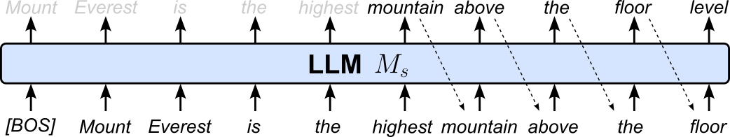
The dashed arrows indicate the iterative process where we add the last predicted token to the context to perform the next forward pass to predict the next token until we have our 5 predicted tokens $w_1$, $w_2$, ... $w_5$ ("mountain above the sea floor"). Overall, we have required 5 forward passes to predict our 5 tokens.
Now we pass the entire sequence $(C, w_1, w_2, \dots, w_5)$ — that is, "Mount Everest is the highest mountain above the sea floor" — to the large model $M_l$. However, the main purpose is not to predict $w_6$ — although we can and will — but to check if $M_l$ agrees with the tokens $w_1$, $w_2$, ... $w_5$ proposed by $M_s$. Recall that we can do this since we get the logits/probabilites for every position in the sequence in parallel. This means we can check which tokens have the highest probabilities for the respective positions using $M_l$, and check if they match the tokens proposed by $M_l$; see the figure below illustrating this step.
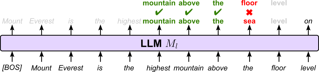
After the complete sequence has been passed to $M_l$ — and we have all required logits/probabilities — we need to check for agreement. If $w_1$ ("mountain") matches $M_l$'s top-1 predicted token for that position, it is accepted. Then we check $w_2$ ("above") — but only if $w_1$ was accepted. We keep checking sequentially until we hit the first mismatch; in our example $w_5$ ("sea" vs. "floor"). Once we hit a mismatch, we combine the current context $C$, all accepted tokens (here: $w_1$, $w_2$, $w_3$) and $M_l$'s prediction of position $4$ ("sea") to form the new context $C$ and the process continues — we pass this new context "Mount Everest is the highest mountain above the sea" to $M_s$ to predict the next five tokens, and use $M_l$ to verify the prediction by checking the agreement between both models. Notice that in our example above, we have an agreement for token $w_5$. However, since we hit a mismatch at $w_4$, we have to ignore all following tokens.
The obvious best case is when both models agree with respect to the whole sequence of predicted tokens. This means that to generate, in our example, 5 tokens, we need 5 forward passes using $M_s$ and only 1 forward pass using $M_l$. If $M_s$ performs significantly faster than $M_l$, this can yield a noticeable improvement in inference speed. On the other hand, if $M_s$ performs very poorly and both models agree on only very few or even no prediction, the overall inference time will actually be longer than using $M_l$ alone. It is therefore important to ensure that both models typically show substantial agreement. For better and more stable results, the basic idea of speculative decoding may also be extended, for example, by deploying multiple smaller models to generate multiple candidate predictions. The overall idea is generally always to minimize the use of $M_l$ and let the smaller but faster models do most of the work.
KV Caching
In LLMs, the autoregressive nature of the Transformer encoder generates text by predicting the next token given a context (i.e., a current sequence of input tokens), adds the newly predicted token to the inputs sequence, and uses this new context as input to predict the next token and so on. The figure below illustrates this process for three iterations for a simple example.
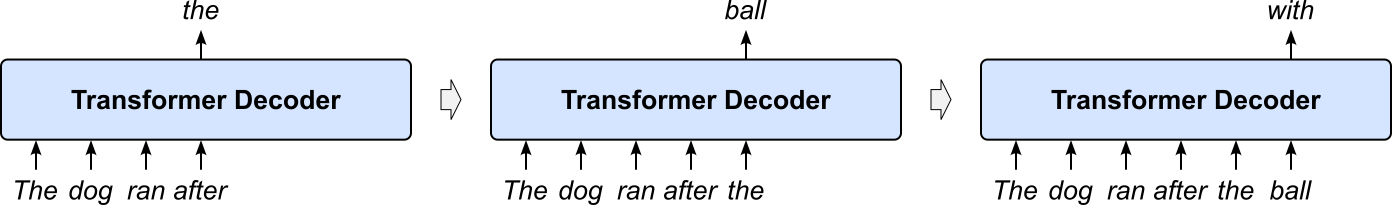
Each iteration (i.e., predicting the next token given the current context) involves a forward pass through all Transformer layers each featuring a Multi-Head Attention (MHA) layer, which itself features multiple Attention Heads. Recall that the output of each attention head is calculated using the following formula:
where $\mathbf{Q}$, $\mathbf{K}$, and $\mathbf{V}$ contain the key, query, and value vectors derived from the sequence of input tokens. The figure below visualizes the attention calculation assuming an input sequence of length $6$ and a size of $64$ for the dimension of the key, query, and value vectors. Note that $\mathbf{QK}^\top$ represents the matrix with attention, and the grey entries reflect the ignored weights after causal masking.
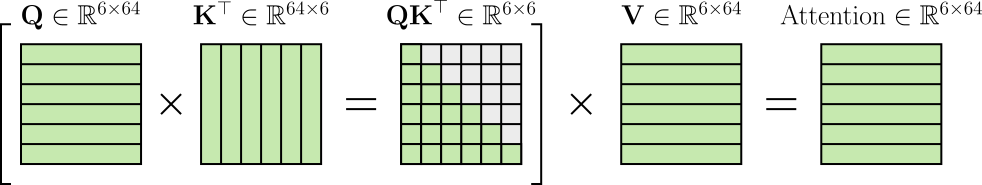
Given this figure it is easy to see that we have to perform computations that we already did before. For example, assuming we started with an initial context of length $3$, we computed the dot product between the first query vector and the first key vector already three — to predict the 4th, 5th, and 6th token. More specifically, given a context of length $t$, to predict the next token, we need the following information
- All key vectors for the previous tokens $w_1$, $w_2$, $w_{t-1}$ [which we also needed in the previous iteration!]
- All value vectors for the previous tokens $w_1$, $w_2$, $w_{t-1}$ [which we also needed in the previous iteration!]
- The query, key, and value vector for token $w_t$
Since we always need the same key and value vectors from the previous iteration, the idea is to simply cache these vectors instead of always recomputing them. Together with the fact that we only need the query vector for token $w_t$ — instead of also the query vectors of all previous tokens — to predict the next token $w_{t+1}$, the attention computation simplifies as shown below:
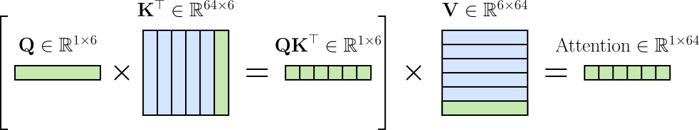
where the blue vectors indicate the key and value vectors taken from the cache, which can significantly speed up the attention computation.
The downside of KV Caching is, of course, that the cache takes up additional memory. Moreover, the cache is growing over each iteration since we always add the most recently computed key and value vector to it. Particularly for long responses generated by the LLM, this can significantly add to the memory footprint of the model.
Reduced model complexity: It is easy to see that the size of the cache depends on the number of Transformer layers, the number of attention heads, and the size of the key and value vectors. By reducing the complexity of the model (e.g., by reducing the number of layers), the size of the memory will also go down. However, reducing the complexity of the model potentially also reduces its performance in terms of quality/accuracy.
Model compression via quantization: Applying quantization to a pretrained model to reduce its overall memory footprint naturally also means that we can quantize the key and value vectors. But as we saw earlier, quantization may also degrade the accuracy of a model.
Modified attention mechanism: The basic attention mechanism computes the alignment between all pairs of tokens individually. Other variants of the attention mechanism aim to minimize the number of involved computations. The section "Efficient Attention" further down below provides more efficiency (but potentially less accurate!) implementations of the attention mechanism.
In short, while there are many ways to reduce the size of the cache introduced by KV Caching, all incur some loss of information which may negatively affect the accuracy of the model. More sophisticated approaches such as modified attention mechanisms also require additional, non-trivial extension to the overall model to perform appropriately. Thus, in practice, KV Caching requires careful consideration of the balance between its benefits and potential downsides.
System-Level Inference Acceleration
Speeding up the inference time of LLMs on a system level generally involves reducing the time it takes for each request to go from input to output by improving hardware efficiency, parallelization, and memory/data handling. Common strategies include:
Hardware support for low-precision operations: With quantization a common way to reduce the memory footprint of a model, optimized processors — most often a GPU, TPU, or specialized accelerator (e.g., NVIDIA Hopper, AMD MI300, Google TPU v4, Intel Gaudi) — have the ability to natively execute arithmetic (like matrix multiplications) on data stored in formats smaller than standard 32-bit floating point (fp32), such as fp16, bf16, int8, or even int4.
Batching and Request Scheduling: Grouping multiple requests to the LLM into a single batch increases GPU throughput, but requires careful scheduling to avoid long waits for smaller queries. Approaches such as dynamic batching adjusts batch sizes on the fly and/or replace completed sequences in a batch with new contexts for optimal latency-throughput trade-offs.
Parallelization and Pipelining: Distributing inference across multiple GPUs or using tensor, pipeline, or sequence parallelism ensures that hardware is always doing useful work. Overlapping computation and communication (e.g., streaming tokens to the client as they're generated) reduces perceived latency.
Memory and I/O Optimization: Reducing CPU–GPU transfer overhead, using pinned memory, preloading models in GPU RAM, and ensuring the inference process is NUMA-aware (non-uniform memory access) can prevent bottlenecks.
Efficient Serving Frameworks: Using specialized inference runtimes (e.g., TensorRT, FasterTransformer, vLLM) that optimize GPU kernel fusion, caching, and memory reuse, etc. can dramatically cut latency. These frameworks can minimize Python overhead, batch requests efficiently, and maximize GPU utilization.
In short, there is a wide range of system-level approaches to accelerate LLM inference, including model quantization, efficient serving frameworks, KV-cache optimization, parallelization, dynamic batching, and memory & I/O tuning. These techniques work together to reduce latency, increase throughput, and make better use of available hardware resources, ensuring that each request is processed as quickly and efficiently as possible. By leveraging specialized hardware support for low-precision operations and optimizing data movement, substantial performance gains can be achieved without changing the model's core architecture. Such optimizations are critical for the practical application and large-scale deployment of LLMs. While training is a one-time cost, inference happens continuously and at scale, directly impacting user experience, infrastructure expenses, and the feasibility of deploying models in latency-sensitive or resource-limited environments.
Efficient Architecture
Efficient architecture design for LLMs means rethinking how the building blocks of Transformers (mainly the attention mechanism but also the feed-forward layers) are structured so that models can scale effectively without incurring prohibitive costs. Instead of relying on the original dense attention mechanism, which grows quadratically with sequence length, researchers design alternatives like sliding-window attention or dilated attention that preserve contextual understanding while reducing complexity. Similarly, architectural choices such as mixture-of-experts layers allow only a subset of parameters to be active for each input, meaning models can be extremely large in capacity but still efficient in practice. These design innovations enable LLMs to process longer sequences, achieve faster inference, and scale to trillions of parameters without linearly increasing computation and memory demands.
Efficient Attention
The basic attention mechanism computes the alignment between all pairs of input tokens/words, resulting in a quadratic time and space complexity. This considerably slows down the pre-training, inference, and fine-tuning of LLMs particularly for long contexts. As a result, various alternative implementations of the attention mechanism have been proposed to reduce its complexity or generally speed-up its computation.
Sharing-based Attention
In standard multi-head attention (MHA) mechanism, each attention head has its own separate, learnable linear projections for the query, key, and value matrices. If there are $n_{heads}$ heads and a hidden dimension of $d_{model}$, this means you have $n_{heads}$ sets of $\mathbf{Q}$, $\mathbf{K}$, and $\mathbf{V}$ matrices, each of size $d_{model}/n_{heads} \times d_{model}$. This results in a total of $3 \times n_{heads} \times (d_{model}/n_{heads}) \times d_{model}$ parameters for the attention block, which is computationally expensive and memory-intensive, especially with large language models. The main benefit is that each head can learn to focus on different parts of the input sequence. The basic intuition behind sharing-based attention mechanisms is to reduce the computational and memory overhead by sharing the key ($\mathbf{K}$) and value ($\mathbf{V}$) projections across multiple attention heads, while still keeping a separate query (Q) projection for each head. This strategy balances the need for diverse attention patterns with efficiency. To popular approaches are:
Multi-Query Attention (MQA): Multi-query attention is the most extreme form of sharing. Instead of having separate $\mathbf{K}$ and $\mathbf{V}$ projections for each head, MQA uses a single set of $\mathbf{K}$ and $\mathbf{V}$ projections that are shared across all heads. The queries, however, still have separate projections for each head. This significantly reduces the number of parameters and the memory required to store the K and V caches during inference. The intuition is that the diverse attention patterns of different heads are primarily captured by the query projections $\mathbf{Q}$. While the key and value projections are important, their function can be largely shared. Sharing them provides substantial efficiency gains during inference because the KV caches (the cached key and value vectors from previous tokens) are much smaller.
Grouped-Query Attention (GQA): Grouped-query attention is a compromise between MHA and MQA. Instead of sharing one set of $\mathbf{K}$ and $\mathbf{V}$ projections across all heads (like MQA), GQA divides the heads into groups and shares a single set of $\mathbf{K}$ and $\mathbf{V}$ projections within each group. This means there are multiple $\mathbf{K}$ and $\mathbf{V}$ projection matrices, but far fewer than in standard MHA. As such, GQA provides a tunable trade-off: you can choose the number of groups ($n_{groups}$) to balance performance and efficiency. If $n_{groups} = n_{heads}$ (the number of heads), it is just basic MHA. If $n_{groups}=1$, GQA is identical to MQA. GQA offers a sweet spot where you get most of the performance of MHA with a significant portion of the efficiency of MQA.
The main challenge of sharing-based attention mechanisms is the loss of expressiveness. In standard MHA, each head has its own keys and values, allowing the model to capture diverse contextual relationships. When keys and values are shared, all heads attend to the same information pool, which can limit the variety of attention patterns the model can represent. This trade-off becomes more pronounced in tasks that require modeling rich, nuanced dependencies (e.g., long-context reasoning or multimodal alignment). Another limitation is that while MQA and GQA greatly improve inference efficiency (especially reducing memory usage during autoregressive decoding), they offer less benefit during training, since training typically computes attention in parallel across tokens and heads. Moreover, if not carefully tuned, these methods may lead to instability in training or degrade accuracy compared to full MHA. In short, sharing reduces redundancy and speeds up inference, but at the risk of lowering flexibility and representational power.
Kernelization or Low-Rank
Looking at the complete formula for the general attention mechanism (see above), let's focus on the part that computes the attention matrix and let's call it $\mathbf{A}$:
A common and useful observation is that $\mathbf{A}$ is often a low-rank matrix. Recall from our idea of low-rank approximation this means that many rows (i.e., attention distributions that sum up to $1$) in $\mathbf{A}$ are nearly linear combinations of others, and that its effective dimensionality is much smaller than the number of tokens $n$. This has several reasons
- Softmax structure: Each row is a probability distribution over tokens. Often, these distributions are highly peaked or repetitive across tokens, leading to redundancy.
- Semantic similarity: Queries/keys for different tokens often live in a low-dimensional manifold. This means their dot products (and hence attention weights) are correlated.
- Redundancy across tokens: Many tokens (e.g., function words, repeated structures) attend in very similar ways, reducing rank.
This observation suggests that the model doesn’t actually need the full $n \times n$ expressiveness of dense attention. The "true" attention patterns occupy a much smaller subspace. Thus, the core idea once again is not to replace $\mathbf{A}$ with a low-rank approximation while preserving most of the model's accuracy. To give a concrete example, the figure below shows the Linformer architecture. The Linformer introduces to additional projection layers $\mathbf{P}_k$ and $\mathbf{P}_v$ to map the key and value vectors into a lower-dimensional space; in the figure below, $\mathbf{K}_p$ and $\mathbf{V}_p$ denote the projected key and value matrices.
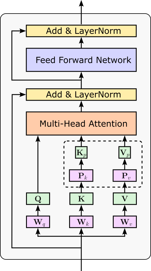
Other low-rank attention strategies similar to Linformer include the Nyströmformer, which approximates the attention matrix using a subset of "landmark" tokens and reconstructs the rest, and Performers, which use random feature maps to approximate the softmax kernel in a low-rank space. Methods like Linear Transformers and Kernelized Attention also rely on projecting queries and keys into lower-dimensional feature spaces so that attention can be computed as a series of low-rank matrix multiplications instead of forming the full $n \times n$ matrix. All of these approaches exploit the empirical observation that attention matrices have rapidly decaying singular values and can be well captured by a smaller rank.
The main challenges with all low-rank strategies are ensuring that the approximation is accurate enough across diverse contexts and sequence lengths. If the rank is too small, important dependencies may be lost, leading to degraded performance. Moreover, while these methods reduce asymptotic complexity, they sometimes underperform dense attention on GPUs/TPUs due to hardware being optimized for dense operations. Balancing approximation quality, stability during training, and actual wall-clock efficiency remains a core difficulty in making low-rank attention practical at scale.
Fixed Pattern Strategies
The basic attention mechanism, where we compute the alignments between all pairs of words/tokens, is also referred to as dense attention. In simple terms, dense attention means the attention mechanism has quadratic complexity of $O(n^2)$, where $n$ is the number of words/tokens in the input sequence. In contrast, sparse attention aims for a linear complexity $O(n)$ by not computing the alignments between all token pairs but only for a selected subset. There are two general strategies how to determine this subset of alignments: fixed pattern strategies and learnable pattern strategies. Let's first look at the idea of fixed pattern strategies.
As the name suggests, fixed pattern strategies confine the attention scope &mash; limiting the number of alignments to be computed — to predetermined patterns. This means that those patterns are not determined as part of the training. Various such predetermined patterns have been proposed. For example, the BigBird sparse attention mechanism combines applies three basic patterns – the figure below visualizes the BigBird approach using a simple example for a question answering data sample:
Local Attention: Each word/token attends to its nearby neighbors within a fixed-sized sliding window. In our simple example below — indicated by the blue boxes — each token attends only to its immediate predecessor and its immediate successor. The intuition is that nearby tokens are typically more useful to describe the meaning of a token than tokens that are farther away. If we denote the size of the sliding window as $w$, the number of attentions is in $O(wn)$, i.e., linear.
Random Attention: Each token additionally attends to a random subset of other token — indicated by the orange boxes. * These sparse, scattered attentions help to avoid the "local-only bottleneck" by providing shortcuts regarding the interaction between arbitrary tokens. Of course, we can easily ensure that the number of random attention is in $O(n)$.
Global Attention: A small set of special words/tokens are designated as global words/tokens; Global tokens attend to all tokens, and all tokens attend to them — notice the green rows and columns in the example below. In principle, any token can become a global token, but a common example are special tokens commonly used during training. For example, the example below contains the "[BOS]" (beginning of sequence) token, the "[SEP]" (separator) token, and the "[EOS]" (end of sequence) token. Global tokens ensure that important positions have "full access" to the whole sequence. Again, if $k$ denotes the number of global tokens, the number of global attention computations is in $O(kn)$.
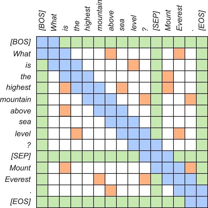
Combining all three patterns means that the total number of attention is in $O(n)$ since we can consider $w$ and $k$ as constants. As such, we can consider BigBird as sparse attention mechanisms. However, it can be shown that BigBird retains the expressive power of dense attention. However, a deeper discussion is beyond our scope here. There are various other approaches similar to BigBird that propose different (combinations of) fixed patterns to implement sparse attention, but all with the same goal: bring down the number of attentions to be computed from $O(n^2)$ down to $O(n)$.
While the potential benefits of sparse attention seem intuitive, there are major practical challenges when actually implementing these mechanisms. GPUs are heavily optimized for dense matrix multiplications (GEMMs — GEneral Matrix Multiply), while sparse attention (as in BigBird) involves irregular access patterns and many "missing" attentions. Naively implementing sparse attention would kill performance on GPUs. Thus, additional strategies are required to actually make sparse attention efficient in practice. For example, BigBird implements block-sparse attention to organize the required data into blocks which can be mapped to block-sparse matrix multiplication, which GPUs handle more efficiently (if supported by the underlying GPU framework). Other proposed strategies involved masking or fusing operations. In short, although the idea of sparse attention strategies seems rather straightforward, their actual implementation is far from trivial.
Learnable Pattern Strategies
Like fixed pattern pattern strategies, learnable pattern strategies aim to implement a sparse attention mechanism by computing only a subset of token alignments. However, the identification of this subset is not done through predetermined patterns but part of the overall learning process. The basic idea is to only compute the alignment that has a noticeable effect on the final output of the attention mechanism and ignore all others. To better understand this, let's have another look at the general attention formula:
Recall that the main concern is $\mathbf{QK}^\top$ which compliments between the alignment between all query and all key vectors, where the number of vectors depends on the input sequence length $n$, thus giving us $O(n^2)$ alignments (i.e., dot products) to compute. Notice, however, that — after scaling — we apply the Softmax function to get the attention weights. The Softmax function ensures that all attention weights are between $0$ and $1$ and that rows of the matrix sum up to $1$. This includes that the small(est) alignment values become attention weights that are close to $0$. Or in other words, if $\mathbf{A}$ denotes the attention matrix, the result of the final step $\mathbf{AV}$ is dominated by the largest attention weights and therefore by the largest alignments.
The idea of learnable pattern strategies is therefore that for each query vector $\mathbf{q}_i$ we only compute the alignments between $\mathbf{q}_i$ and the key vectors yielding the largest values — of course, without the need to compute all alignments to find the largest values! Since we compute the alignment between tokens using the dot product, the alignment is largest if the corresponding query and key values are similar — point roughly in the same direction (assuming that the magnitudes are generally similar). In short, we only consider pairs of query and key vectors with similar vectors. Many such strategies have been proposed; let's very briefly look at two ideas to get the gist:
Locality Sensitive Hashing (LSH): LSH is a technique used to efficiently find similar items (e.g., vectors) in high-dimensional spaces. To this end, LSH uses specially designed hash functions that maximize the chance of placing similar items into the same hash bucket to quickly narrow down the search space for approximate nearest neighbor queries. Applied to the attention mechanism, the idea is to assign each token to a bucket using an LSH. Because LSH has the property that similar vectors are likely to hash into the same bucket, tokens with similar representations (and thus likely relevant to each other) are grouped together. Then, self-attention is computed only within each bucket (and possibly a small number of nearby buckets). This dramatically reduces the complexity from quadratic $O(n^2)$ to nearly linear $O(n \log n)$.
Clustering: Clustering is an unsupervised learning technique that groups data points (e.g., vectors) into clusters such that points within the same cluster are more similar to each other than to points in other clusters. In the context of sparse attention for LLMs, clustering can be used to organize tokens into groups based on their hidden representations. Instead of letting every token attend to every other token (which costs $O(n^2)$), the model first clusters tokens. Attention is then computed only within clusters and, optionally, across a few neighboring or representative clusters. This way, tokens that are semantically or contextually similar are grouped together, and attention is restricted to these subsets. Again, the complexity is reduced to something closer to $O(n \log n)$ or even linear, depending on the clustering strategy. This approach is similar in spirit to LSH attention (which uses randomized hashing), but clustering is typically deterministic and data-driven.
LSH and clustering (as well as similar approaches) add their own additional overhead to the attention mechanism. However, the overall reduction of complexity from $O(n^2)$ to typically $O(n\log n)$ generally justifies the added steps. Of course, like with fixed pattern strategies, sparse attention mechanisms using learnable pattern strategies also have to ensure that the mechanism is indeed implemented efficiently — as most GPU frameworks are only optimized for dense matrix multiplications.
Hardware-Assisted Attention
Hardware-assisted attention computation refers to a set of techniques and algorithms that leverage the specific architecture of computer hardware, such as GPUs, to make the attention mechanism in LLMs more efficient. The core idea is to move the computation of attention from being a memory-bound operation to a compute-bound one. At a high level, the basic ideas behind hardware-assisted attention computation revolve around minimizing data movement and optimizing the computational flow to better utilize the hardware's capabilities.
Minimizing Data Movement (IO-Awareness): The standard attention mechanism in an LLM is often bottlenecked by the need to constantly move large amounts of data (specifically the query, key, and value matrices) between different memory hierarchies. A GPU has a fast, but small, on-chip memory (SRAM) and a slower, but large, High Bandwidth Memory (HBM). The main bottleneck is the frequent reading and writing of intermediate matrices, like the attention scores, from the slow HBM. Techniques such as FlashAttention address this by reorganizing the computation. Instead of performing the entire attention calculation in a single step that requires loading everything into HBM, it breaks the process down into smaller "tiles". The computation for each tile is performed entirely within the fast on-chip memory (SRAM), and the intermediate results are not written back to HBM until the entire attention block is computed. This significantly reduces the slow and energy-intensive data transfer, leading to substantial speedups.
Reordering and Fusing Operations (Kernel Fusion): Recall that the attention mechanism consists of a series of operations: (1) computing the dot product between $\mathbf{Q}$ and $\mathbf{K}$, (2) scaling the result $\mathbf{QK}^\top$, (3) applying the Softmax function to get the attention weights, and (4) computing the dot product between the attention weights and $\mathbf{V}$. In a naive implementation, each of these steps might be a separate "kernel", or program, run on the GPU. This means data is loaded for step one, the results are stored, then the results are loaded again for step two, and so on. This introduces significant overhead. Hardware-assisted methods fuse these operations into a single, cohesive kernel. This means the entire attention calculation is performed in one go without the need to save and load intermediate results between steps. By fusing these kernels and using techniques like online softmax, the process becomes a single, highly optimized block of code that runs on the GPU's compute units, maximizing their utilization and reducing latency.
Due to their relevance in importance given the popularity of LLMs, hardware-assisted attention computation encompasses a variety of techniques designed to boost the efficiency of Large Language Models by optimizing their performance on specialized hardware like GPUs. Although different methods exist, they generally fall under two aforementioned core strategies.
Mixture of Experts (MoE)
In a traditional neural network — including the original Transformer architecture — every input is processed through all layers of the network, and each layer consists of a fixed set of neurons with associated weights and biases (i.e., the trained parameters). These parameters are not conditionally activated or skipped during inference, meaning all parameters are used regardless of the input for both training and inference. This means that the computational cost increases proportional to the capacity of the model (expressed as the number of trainable parameters).
An alternative paradigm are sparsely activated model where only a subset of parameters might be used for a given input — again, during training and inference. The most common type of sparsely activated model is the Mixture of Experts (MoE), often used as a component or layer as part of a Transformer model. A basic MoE model consists of two main components — see also the figure below:
Set of Experts: An expert $E_i$ is "some" separate subnetwork — typically a simple Feed-Forward Network (FFN), but it can be any architecture — that processes an input $\mathbf{x}$. A MoE model typically consists of dozens or even hundreds of experts, either of the same type (homogeneous experts) or of different types (heterogeneous experts). The final output of the MoE model is calculated as the weighted sum of the outputs of all activated experts. The weights of the sum as well as the set of activated experts is determined by the gating mechanism. In the figure below, we assume that we have $n$ experts $E_1$, $E_2$, ..., $E_n$, and the input is passed to $2$ selected experts.
Gating Mechanism: The gating mechanism is a submodel — again, typically an FFN — that determines to which experts input $\mathbf{x}$ should be passed to. Its output is a probability distribution over all experts $G(\mathbf{x})$, and input $\mathbf{x}$ is passed to the experts $E_i$ with the highest probabilities $G(\mathbf{x})_i$. We can distinguish between two components in the gating mechanism (although they are often considered together). The Gate submodel calculates the initial distribution $G(\mathbf{x})$. The Router submodel then uses $G(\mathbf{x})$ to determine to which experts the input should be passed based on various routing strategies; this may include a rescaling of the probabilities if only a subset of experts are involved in the final output.
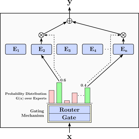
The parameters in both the experts and the gating mechanism are learned during the training. Given this overall architecture setup, the output $\mathbf{y}$ of an MoE model is calculated as:
Where $E_i(\mathbf{x})$ is the output of expert $E_i$ given the input $\mathbf{x}$. The interesting case is where $G(\mathbf{x})_i = 0$ for an expert $E_i$, either because the gate probability is already $0$ or is set to $0$ as part of a routing strategy. For example, the figure above illustrates the routing strategy that sends input $\mathbf{x}$ to only the two experts with the highest probabilities calculated by the gate. To accomplish this, all other probabilities are set to $0$ — indicated by the red bars of the probability distribution — the remaining two probabilities are rescaled to again sum up to $1$ (green bars). Naturally, for any $G(\mathbf{x})_i = 0$, there is no need to pass the inputs to the respective expert $E_i$. In short, for this and similar routing strategies, only a part of the overall network is activated and utilized.
When it comes to the routing strategies, there are two basic alternatives. In a dense MoE model, an input $\mathbf{x}$ is passed to all experts, and all their outputs are part of the weighted sum to calculate $\mathbf{y}$. In other words, generally, $\forall i: G(\mathbf{x}_i) > 0$. This makes dense MoE models very easy to implement since no actual routing in terms of selecting individual experts is performed. Dense MoE models therefore do not require a dedicated router component, and only rely on the probability distribution as the output of the gate. However, activating all experts for every input undermines one of the original motivations of MoE architectures — to achieve high capacity without linearly increasing computation. As a result, dense MoE models can become prohibitively expensive for large-scale deployments, especially in environments with limited resources or strict latency constraints. Another downside is the potential for redundancy among experts.
In contrast, in sparse MoE models, an input $\mathbf{x}$ is typically no longer passed to all experts. In contrast, different training samples may be passed to different subsets of experts. This generally makes implementing sparse MoE models more challenging as compared to dense MoE models. This also includes that the sparse MoE models feature a router that implements a specific routing strategy that decides which training samples get passed to which experts. A common implementation of a router is top-k router, where $k$ refers to the number of experts a training sample is passed to. In a nutshell, the router takes as input the gate probabilities and performs two basic steps. It first identifies the top-$k$ probabilities $G(\mathbf{x})_i$ for each training sample as the well indices of the corresponding exports. The router then updates the gate probabilities by (a) setting the probabilities of all experts a training sample is not passed to $0$, and (b) recalculates the probabilities of the remaining top-k experts so that the sum up to $1$ again. Note that this simple implementation does not feature any trainable parameters.
Despite their advantage with respect to computational efficiencies, sparse MoEs models come with several challenges. One of the biggest is load balancing — that is, ensuring that all experts are utilized evenly. Without careful design, some experts may be overused while others are rarely activated, leading to undertrained parts of the model and degraded performance. Techniques like auxiliary loss terms or routing constraints are often needed to encourage balanced usage of experts, which adds complexity to the training process. Another major difficulty is routing — deciding which experts to activate for a given input. This is typically done via a learned gating mechanism, which must be efficient and differentiable. The routing introduces discrete choices that can make training harder to optimize using gradient-based methods. Lastly &mdash' as we could already see in our basic example implementation — implementation and deployment complexity is higher for sparse MoE models. They require dynamic computation graphs and often non-standard memory access patterns, which can be difficult to scale efficiently on GPUs or in distributed systems. This makes sparse MoEs powerful but also technically demanding to use in practice.
Long Context LLMs
LLMs are typically trained on inputs with a fixed maximum length because it simplifies both computation and memory management during training. Transformer-based models process sequences in parallel using attention, where the computational and memory cost grows quadratically with sequence length. By fixing a maximum length, training can be standardized into batches of equal size, making it more efficient to run on GPUs/TPUs and avoiding highly variable resource usage that would arise if each input had an arbitrary length. Shorter sequences are padded to the fixed size, while longer ones are truncated, ensuring uniformity.
In practice, however, there are several important applications where LLMs often need to handle sequences much longer than what they were trained on. A common one is document understanding and summarization, where real-world texts like legal contracts, research papers, or books far exceed the usual training limits (e.g., 2k-4k tokens). Similarly, code understanding and generation often requires processing entire repositories or long source files, which can go well beyond the model's training context. Another major case is multi-turn dialogue and conversational agents, where conversations accumulate context over time and can surpass the training limit if the history is kept in full. In retrieval-augmented generation (RAG) and question answering over knowledge bases, large amounts of retrieved text may need to be processed in a single pass. Other domains where inputs can be extremely long include, log analysis, biomedical records, and financial reports.
A straightforward way to solve this problem is to fine-tune LLMs on data with long sequences, but this again takes a lot of time and computing power. To make things more efficient, new methods have been proposed to help LLMs handle longer inputs without such heavy costs. These methods generally fall into four groups: extrapolation and interpolation, recurrent structures, segmentation with sliding windows, and memory or retrieval-based augmentation. Let's have a look at their fundamental ideas.
Positional Extrapolation and Interpolation.
Recall that Transformer-based LLMs need positional encodings because, unlike models such as RNNs, they process all tokens in a sequence at the same time and have no built-in sense of order. Without extra information, the model would see a sentence as just a bag of tokens, ignoring the fact that word/token order changes meaning. Positional encodings solve this by giving each token a numerical signal that represents its position in the sequence, allowing the model to understand both the order of tokens and their relative distances.
The figure below shows one of the basic ways to incorporate positional encodings — and as proposed and applied in the original Transformer architecture. In this figure, $\mathbf{w}_i$ represents the embedding vector of the word/token at the $i$-th position in the input sequence of length $L$; $\mathbf{p}_i$ is an embedding vector encoding position $i$ which is added to token embedding vector $\mathbf{w}_i$, forming the combined embedding vector $\mathbf{e}_i$. The result vectors then form the input sequence for the Transformer model.
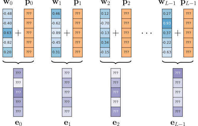
Many positional encoding strategies have been proposed that differ not only with respect of how the positional encoding vectors $\mathbf{p}_i$ are computed but also how they are incorporated as part of the training — for example, some approaches add positional information as part of the attention mechanism itself.
Some encoding strategies allow to create meaningful vectors $\mathbf{p}_i$ for positions larger than the model has seen during training. For example, fixed positional encodings are position signals that are predefined and do not change during training. A common example is the sinusoidal encoding used in the original Transformer, where each position in the sequence is mapped to a combination of sine and cosine functions at different frequencies. This allows the model to extrapolate positional encodings beyond positions seen during training. However, approaches such as the sinusoidal encoding still often underperform on sequences longer than those seen in training because the model has not been exposed to the patterns of how these encodings interact with attention, so it may fail to interpret them meaningfully. Thus, more sophisticated techniques are needed. For example, ALiBi (Attention with Linear Biases) avoids giving tokens explicit positional embeddings and instead adds a simple bias directly to the attention scores that depends on the distance between tokens. This encourages the model to focus more on nearby tokens while still allowing it to attend to distant ones if useful. Still, encoding strategies that allow for extrapolation — at least in principle — still show a drop in performance at some point when working with long(er) inputs.
An alternative approach is trying to interpolate positional encodings. The basic idea here is to rescale the positional signals learned during training so they can be reused at longer sequence lengths. For example, if a model was trained with embeddings for positions up to 2k tokens, interpolation stretches or compresses these embeddings so they can cover, say, 8k tokens. Interpolation works with relative positional encodings where the positional encoding vectors do not capture the absolute position of tokens but their relative positions, i.e., the distance between tokens. If stretching or compressing do not affect the relative distances between tokens, by smoothly adjusting the learned encodings, the model can generalize its understanding of position to longer contexts without needing to be retrained from scratch. While stretching or compressing the positional encodings does change the exact numerical values of relative distances, Transformer models usually do not rely on precise absolute distances; instead, they learn broad patterns of locality and relative positioning during training (e.g., "nearby tokens are more related than very distant ones"). When the encodings are rescaled, these relative patterns are approximately preserved, even if the exact values shift.
Recurrent Structure
A very naive way to handle inputs longer than the ones seen during training would be to simply split the input into segments, where each segment's length matches the maximum sequence length during training. Naturally, this would avoid any issues with unseen/unknown positional encodings. The figure below illustrates the idea; the final output would be the concatenation of the individual outputs for each segment.
However, it is easy to convince yourself that this naive approach is unlikely to perform well in practice, since the processing of a segment is completely independent from all previous segments. For example, the output for segment $t+1$ is not affected by all precious segments $1$, $2$, ..., $t$. This is a problem as the original (long) context assumingly was a coherent text that was now split into independent segments. One possible solution is therefore to introduce some kind of memory that captures the processing of previous segments and then serves as an additional input of the current segment; see the figure below illustrating the overall idea.
This idea of a memory is similar in spirit to Recurrent Neural Networks (RNNs) that maintain a memory of previous tokens to influence future predictions. In RNNs, the memory is a hidden state that is updated sequentially at every time step, i.e., at each token. A popular Transformer-based architecture that adopts this idea is the Transformer-XL model, which caches the hidden states from previous segments and reuses them as additional context for the current segment. This allows the model to capture dependencies that span beyond the fixed maximum length used during training, effectively giving it a much longer receptive field without needing to increase the input size at once. In short, while RNNs rely token-level recurrence, Transformer-XL (and similar architecture) utilize segment-level recurrence.
More specifically, the hidden state refers to the output representations of each token from a Transformer layer in a given segment. After processing a segment of tokens, each layer produces a set of hidden vectors (one per token) that encode both the token’s content and its contextual relationships within that segment. To integrate these hidden states into the next segment, Transformer-XL caches them as a "memory". When the next segment is processed, the attention mechanism can attend not only to tokens in the current segment but also to these cached hidden states from previous segments — in more detail, the hidden stated is concatenated to the current key and value matrices (but not the query matrix) for the attention computation. Importantly, the cached states are detached from the gradient computation, meaning they are treated as fixed inputs rather than being updated again during backpropagation for the new segment. This allows the model to extend its effective context across segments efficiently, without recomputing or storing gradients for the entire long sequence.
Note that the Transformer-XL model also requires relative positional encodings, since the absolute positional encodings for different would be identical. Transformer-XL and similar architectures also face memory management and computational overhead. While caching hidden states allows the model to access long-range context without recomputing previous segments, it still requires storing multiple layers' worth of hidden states for potentially many past segments. Another limitation is gradient flow and learning dynamics. Since the cached hidden states from previous segments are detached from the gradient during training, the model cannot backpropagate through them. This prevents the network from directly learning to correct errors in long-range dependencies across segment boundaries. In effect, the model must learn to predict based on partial, non-trainable memory, which can reduce its ability to fully exploit very long contexts compared to training on fully contiguous sequences. Finally, sequence segmentation introduces boundary effects may cause tokens near the boundary between segments to receive less precise context, especially if important dependencies span the split. While the memory mitigates this, it does not completely eliminate the problem, and the model may underperform on tasks requiring precise long-range reasoning.
Segmentation and Sliding Window
Sliding window approaches implement a sparse attention mechanism like we have seen before to cap the maximum required memory when computing attention even for very long sequences. Again, the underlying idea is to calculate the attention weights for only a subset of token pairs instead of for all pairs. To this end, a basic slides window approach — for example as done by the Mistral LLM — only computes the weights for a token and its $k$ preceding token; notice that we only consider preceding tokens since Mistral is a decoder-only LLM and therefore applies causal masking as part of the autoregressive text generation.

A sliding window reflects the intuition that nearby tokens are typically more indicative for the meaning or importance of a current token. It is important to note, however, tokens outside/before the sliding window still affect a token. This is due to the fact that the Transformer decoder has multiple layers. Each Transformer layer in Mistral only lets a token attend to its local window (say, just 4 tokens given our toy example above). But when stacking multiple layers, information from farther away can "hop" across layers. Let's look at an example using small window size of 4
Layer 1: token at position 20 can attend to tokens 16 - 19.
Layer 2: token at position 20 now has access to information from 12–19, because tokens 16–19 already aggregated their own neighborhoods.
Layer 3: token at position 20 now has access to information from 8–19, because tokens 12–19 already aggregated their own neighborhoods.
Layer 4: ...
The decoder only needs enough layers that a token has access to the information from the first token onwards. This is typically ensured since the sliding window is in practice much larger (e.g., several hundreds or thousands of tokens), and the larger the sliding window the less layers are needed. Mistral also uses KV Caching to improve efficiency. Of course, this cache only stores the key and value vectors for the tokens in the within the sliding window, and therefore all cache entries must be removed after each predicted token.
A very similar sliding window approach is proposed by the StreamingLLM model. The build upon the observation that the very few first tokens very often seem to be very important to ensure a model's accuracy. Since a normal sliding window approach would at some point stop attending to the very first tokens — at least directly attending and not indirectly across multiple Transformer layers — StreamingLLM preserves the key and value vectors of the very first tokens always in the cache. The figure below adopts the previous example by including the computed attention weights between tokens and the, here, first two initial tokens.
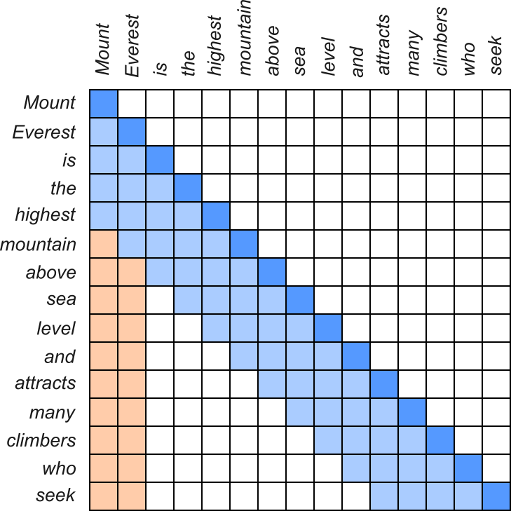
Beyond Mistral and StreamingLLM, other architectures have been proposed that implement some form of sparse attention to efficiently handle very long contexts. For example, The LongNet Transformer extends Transformers to handle up to millions of tokens by replacing standard dense attention with dilated sliding-window attention. Instead of attending to all tokens or just a fixed local window, each layer uses a dilated pattern: tokens attend to others at increasing intervals (e.g., every 2nd, 4th, 8th token), so higher layers connect distant parts of the sequence efficiently. The Parallel Context Windows (PCW) split the input sequence into overlapping windows that can be processed in parallel. Each window has its own attention computation, ensuring local coherence, while the overlaps allow information to flow across boundaries. After parallel processing, the outputs are combined so that tokens near window edges can still integrate context from neighboring windows.
Memory-Retrieval Augmentation
Since the hidden state of recurrent architectures is some form of memory, the Transformer-XL and similar architectures are examples of memory-retrieval augmentation. However, memory-retrieval augmentation can be more generalized to any kind of approaches that keep some kind of information that is added, typically to the key and value matrices which represent the context within the attention mechanism. Architectures using memory-retrival augmentation have to address two main considerations:
Caching strategy: The caching strategy determines which information is kept within the memory. For example, the Transformer-XL model keeps all the hidden states from all the layers from the previous segment. Other common strategies focus on identifying tokens or representations that are salient, compressible, or likely to be needed later. One approach is to use learned attention or gating mechanisms to detect which tokens strongly influence predictions, while simpler heuristics might select special tokens, segment boundaries, or embeddings that summarize important content. Another set of strategies involves compression or aggregation, where multiple tokens are combined into a single memory representation, preserving key information without overloading memory. Additionally, some methods use retrieval-driven selection, storing content that is predicted to be relevant for future queries based on similarity or relevance scoring. In practice, these strategies are often combined, allowing the model to efficiently capture long-range dependencies while keeping memory usage manageable.
Retrieval strategy: Once we have some information in our memory, we now have to decide which parts we use for the processing. Again, recall that the Transformer-XL architecture uses the complete memory as it represents this hidden state from the previous segment. A common alternative strategy is attention-based retrieval, where the model computes attention scores between the current input and memory keys, weighting memory entries by their relevance. Similarly, similarity-based retrieval** uses metrics (e.g., dot product, cosine similarity, k-nearest neighbor) to select memory slots most similar to the current query. More advanced approaches include learned retrieval modules, where a neural network predicts which memory entries are likely to be useful, and hierarchical or clustering-based methods, which organize memory into groups to quickly narrow down relevant information. Often, these strategies are combined, allowing the model to first filter the memory and then dynamically attend to the most relevant entries.
Obviously, memory-retrieval augmentation strategies require additional memory management: storing and retrieving large numbers of key-value pairs can be computationally expensive and memory-intensive, especially as the external memory grows. This can create bottlenecks during training and inference, and may limit the practical length of context the model can handle. Another limitation is retrieval quality. If the memory selection or retrieval mechanism fails to identify the most relevant information, the model may attend to unhelpful or redundant entries, reducing performance. Additionally, these strategies often require extra components or learned modules, adding complexity to the model and potentially making training more difficult. Finally, there is a risk of information drift: since memory is usually updated incrementally, older or less frequently accessed content may become stale or less reliable, which can affect the model’s consistency and accuracy over very long contexts.
Transformer-Alternative Architectures
At the time of writing (August 2025), The Transformer architecture is (still) default choice for training large language models (LLMs) because it provides an efficient and scalable way to process sequential data. Its use of the attention mechanism allows the model to capture dependencies between any pair of tokens in a sequence, regardless of distance, which earlier recurrent or convolutional approaches struggled with. Just as importantly, the design eliminates sequential bottlenecks, enabling highly parallelized training that fits modern hardware accelerators. Over time, Transformers have demonstrated unmatched versatility and performance, becoming the foundation for nearly all state-of-the-art LLMs. Their scalability to billions of parameters, combined with adaptability through architectural refinements and fine-tuning methods, has solidified them as the default architecture for advancing natural language processing.
On the other hand, the attention mechanism at the heart of the Transformer also poses challenges particularly in terms of efficiency — hence the wide range of approaches outlined in this notebook to make LLMs more efficient. The attention mechanism computes the alignment between all pairs of tokens (ignoring masking) at the same time. While this results in complexity of $O(n)$, with $n$ being the number of input tokens, it does allow for a straightforward parallelization during training. However, when generating the next token during inference, we need to recompute the attention for the entire sequence, even if we already generated some tokens. While this repeated computation were the main motivation behind strategies such as KV caching, they do come with significant memory overhead — and counter-strategies such as multi-query attention (MQA) and grouped-query attention (GQA) may risk a degradation of the models's accuracy.
In fact, in terms of inference efficiency, Recurrent Neural Networks (RNNs) had a clear advantage. Recall that an RNN is a sequential model architecture that reads in an input token by token and updates an internal hidden state. While this prohibits the parallel processing of sequence during training, the generation of tokens during inference is much more efficient. Here, the prediction of the next token only depends on the current hidden state and the current input (i.e., the last predicted tokens in the case of inferencing). Notice that this does not involve any repeated computations — and in general also much less computations. The main limitation of RNNs (and more sophisticated variants such as LSTMs and GRUs) is — and this was the main motivator for the Transformer architectures — that the hidden state needs to capture the complete sequence of tokens. In practice, RNNs start to "forget" early tokens when working with long sequences — in other words, early tokens were no longer captured by the hidden state.
One of the more promising alternatives for the Transformer architecture are State Space Models (SSMs). Like Transformers and RNNs, SSMs process sequences of information. And like RRNs, SSMs feature and update an internal state which greatly improves inference efficiency. Also SSMs update the internal state using linear operations, compared to RNNs that perform nonlinear operations. This makes information flow more stable and structured, allowing SSMs to retain and propagate signals across much longer contexts. The application of SSMs for language modelling is far from trivial, though:
Continuous vs discrete data: SSMs describe sequences using continuous-time dynamics, typically through systems of linear differential (or difference) equations that evolve a hidden state over time. For language modeling, modern neural SSMs need to discretize these equations efficiently and combine them with learned parameters.
Complex Dependencies: Natural language involves hierarchical, compositional, and cross-token relationships (e.g., syntax, coreference). SSMs naturally excel at sequential memory and long-range signal propagation, but they are less straightforward in capturing flexible pairwise interactions compared to attention, which can directly relate any two tokens.
Time-invariance and selectivity: Classical SSMs are time-invariant and lack selectivity. For language modeling, this makes it difficult for SSMs to selectively focus on or ignore specific parts of the input, which is crucial for handling the dynamic nature of language. Thus, modern architectures like Mamba introduce selective state space models that can dynamically choose which information to pass to its state and which to ignore, effectively simulating a context-aware mechanism similar to attention but with a linear scaling property.
Beyond State Space Models (SSMs), other architectures have been proposed to potentially Transformer models. In essence, most of them try to combine the advantages of Transformers (capturing of long-term dependencies and parallel training) and Recurrent Neural Networks (efficient inference). For the time being, however, Transformer-based LLMs still outperform existing alternatives. The main reason for that is because the attention mechanism is more effective at capturing more complex and nuanced dependencies between tokens.
Data-Centric
Coming soon...
Data Selection
Data Selection for Efficient Pre-Training
Data Selection for Efficient Fine-Tuning
Prompt Engineering
Few-Shot Prompting
Prompt Compression
Prompt Generation
Summary
The rapid success of Transformer-based large language models (LLMs) has created both opportunities and challenges. Their ability to model long-range dependencies and scale to billions of parameters has made them the foundation of modern AI systems, but this comes at a steep computational and memory cost. Training and inference of such models require enormous GPU clusters, large amounts of energy, and optimized software pipelines. As a result, the research community has devoted significant effort to finding strategies that make both training and inference more efficient without sacrificing model performance.
One major line of work focuses on attention efficiency. Since standard self-attention scales quadratically with sequence length, researchers developed sparse and structured attention mechanisms like sliding window attention (Mistral), dilated attention (LongNet), or hybrid local-global schemes (Longformer, BigBird). These methods reduce computation while ensuring that long-range information can still propagate. Others explored low-rank approximations (Linformer, Performer) and memory retrieval strategies, all designed to extend context length while keeping complexity closer to linear. Such techniques directly address the bottleneck of processing long sequences, which is central to both training large corpora and serving real-world applications.
Another area of innovation targets model efficiency. Techniques like parameter sharing, quantization, pruning, and low-rank adaptation (LoRA) reduce the memory footprint and computational overhead. For training, optimizers and distributed training strategies (ZeRO, tensor parallelism, pipeline parallelism) allow scaling across thousands of GPUs while keeping memory usage manageable. These advances make it possible not only to train trillion-parameter models but also to adapt them efficiently to specialized domains without retraining from scratch.
Finally, inference efficiency has become just as important as training. Strategies such as KV Caching, speculative decoding, and efficient batching greatly reduce latency and resource requirements when deploying LLMs in interactive applications. Hardware-aware optimizations, like custom GPU kernels and support for low-precision operations, further accelerate inference. Together, these innovations ensure that LLMs can be deployed at scale for tasks ranging from chatbots to code assistants, making them practical for widespread use.
To sum up, the dominance of Transformer-based LLMs has spurred a wide spectrum of efficiency strategies spanning architecture design, training methods, and inference optimizations. Each strategy addresses a different bottleneck—attention complexity, parameter scaling, or serving latency—reflecting the diverse challenges of scaling these models to real-world demands. The interplay of these techniques has enabled the rapid growth of the LLM ecosystem, making it feasible to train and serve ever-larger models that continue to redefine the state of the art.