Disclaimer: This Jupyter Notebook contains content generated with the assistance of AI. While every effort has been made to review and validate the outputs, users should independently verify critical information before relying on it. The SELENE notebook repository is constantly evolving. We recommend downloading or pulling the latest version of this notebook from Github.
Mixture of Experts (MoE)
In deep learning, the Mixture of Experts (MoE) model is a powerful architectural technique that enhances model efficiency by dynamically selecting specialized sub-networks — or "experts" — for different input data. Instead of relying on a single monolithic neural network to process all types of inputs, MoE divides the computational workload among multiple smaller networks, each trained to handle specific patterns or distributions. A gating network determines which experts to activate for a given input, ensuring that only the most relevant ones contribute to the final prediction.
One of the key advantages of MoE is its ability to scale model capacity without a proportional increase in computation cost. Since only a subset of experts is active for each input, the model can maintain high expressiveness while keeping inference computationally efficient. This makes MoE particularly beneficial for large-scale applications, such as natural language processing (NLP), speech recognition, and computer vision, where diverse patterns exist within the data. Google's Switch Transformer and other large-scale language models have leveraged MoE to improve performance while managing computational overhead.
Another major benefit of MoE is its adaptability to heterogeneous data distributions. In real-world tasks, data often follows a multi-modal distribution, meaning different sub-populations require specialized processing. MoE naturally captures this by allowing different experts to learn distinct aspects of the data. This approach improves generalization and reduces the risk of overfitting, as each expert focuses on a more manageable subset of the data distribution rather than attempting to generalize across all possible inputs.
Despite its advantages, MoE also introduces challenges, such as training instability and load balancing issues among experts. If the gating network assigns most inputs to a small subset of experts, the model may fail to utilize its full capacity. Researchers have proposed techniques like regularization, auxiliary losses, and improved gating mechanisms to mitigate these issues. Overall, the MoE layer is a powerful tool for improving the scalability and efficiency of deep learning models, making it a popular choice for modern AI architectures.
Setting up the Notebook
Make Required Imports
This notebook requires the import of different Python packages but also additional Python modules that are part of the repository. If a package is missing, use your preferred package manager (e.g., conda or pip) to install it. If the code cell below runs with any errors, all required packages and modules have successfully been imported.
import torch
import torch.nn as nn
import torch.nn.functional as F
Generate Example Data
Throughout this notebook, we illustrate the basic idea of an MoE layer and its inner works using a small example batch that forms the input for the MoE layer. To keep it simple, the batch contains $4$ data samples, each sample represented by a vector of size $8$.
batch_size, hidden_size = 4, 8

torch.manual_seed(0)
batch = torch.rand((batch_size, hidden_size))

print(batch)
tensor([[0.4963, 0.7682, 0.0885, 0.1320, 0.3074, 0.6341, 0.4901, 0.8964],
        [0.4556, 0.6323, 0.3489, 0.4017, 0.0223, 0.1689, 0.2939, 0.5185],
        [0.6977, 0.8000, 0.1610, 0.2823, 0.6816, 0.9152, 0.3971, 0.8742],
        [0.4194, 0.5529, 0.9527, 0.0362, 0.1852, 0.3734, 0.3051, 0.9320]])
MoE: Basic Model Architecture
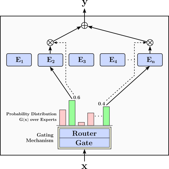
To give a first overview, the figure below illustrates the basic architecture of a Mixture-of-Experts model. This architecture feature two main components:
Experts: The experts are separate networks that process the input $\mathbf{x}$. The final output of the MoE model is calculated as the weighted sum of the outputs of all activated experts. The weights of the sum as well as the set of activated experts is determined by the gating mechanism. In the figure below, we assume that we have $n$ experts $E_1$, $E_2$, ..., $E_n$, and an input $\mathbf{x}$ is passed to $2$ selected experts.
Gating Mechanism: The gating mechanism is a submodel that determines to which experts input $\mathbf{x}$ should be passed to.
Its output is a probability distribution over all experts $G(\mathbf{x})$, and input $\mathbf{x}$ is passed to the experts $E_i$ with the highest probabilities $G(\mathbf{x})_i$. We can distinguish between two components in the gating mechanism (although they are often considered together). The Gate submodel calculates the initial distribution $G(\mathbf{x})_i$. The Router submodel then uses $G(\mathbf{x})_i$ to determine to which experts the input $\mathbf{x}$ should be passed based on various routing strategies; this may include a re-scaling of the probabilities if only a subset of experts are involved in the final output.
The parameters in both the experts and the gating mechanism are learned during the training.
Given this overall architecture setup, the output $\mathbf{y}$ of an MoE model is calculated as:
Where $E_i(\mathbf{x})$ is the output of expert $E_i$ given the input $\mathbf{x}$. The interesting case is where $G(\mathbf{x})_i = 0$ for an expert $E_i$, either because the gate probability is already $0$ or is set to $0$ as part of a routing strategy. For example, the figure above illustrates the routing strategy that sends input $\mathbf{x}$ to only the two experts with the highest probabilities calculated by the gate. To accomplish this, all other probabilities are set to $0$ — indicated by the red bars of the probability distribution — the remaining two probabilities are re-scaled to again sum up to $1$ (green bars). Naturally, for any $G(\mathbf{x})_i = 0$, there is no need to pass the inputs $\mathbf{x}$ to the respective expert $E_i$. In short, for this and similar routing strategies, only a part of the overall network is activated and utilized.
MoE: Core Components
While MoE models can become quite complex in practice, they typically all feature the same basic core components.
Experts
An expert in the context of a Mixture-of-Expert layer is a subnetwork or submodel within a larger model. Each of these subnetworks independently perform their own computation, and their results combined to create the final output of the MoE layer. In principle, an expert subnetwork can be any kind of architecture but are commonly simple ones such as basic feed-forward neural networks (FFNNs). To give an example, the code cell below implements a very simple expert as a FFNN with two linear layers. The first linear layer transforms the input of size hidden_size into a higher dimensional space (here: hidden_size*4). After applying the ReLU activation function, the second linear layer transforms the result back to initial input size. As a side note: this expert mimics the FFNN layer in the transformer architecture.
class Expert(nn.Module):

    def __init__(self, hidden_size):
        super().__init__()
        self.net = nn.Sequential(
            nn.Linear(hidden_size, hidden_size*4),
            nn.ReLU(),
            nn.Linear(hidden_size*4, hidden_size)
        )

    def forward(self, x):
        return self.net(x)
Traditionally, most MoE models use homogeneous experts — that is, each expert uses the same architecture and therefore has the same capacity. In contrast, MoE models with heterogeneous experts rely on different architecture for the set of experts. While this heterogeneity allows for more specialized experts — -- which can be very useful when working with multimodal data (e.g., text & images) or multitask learning, training MoE models heterogeneous experts are generally more complex and more difficult to train. In this introduction notebook, we therefore limit ourselves to homogeneous experts.
With our Expert class implementation, we can create an expert subnetwork as shown in the code cell below. Of course, we specify the input size of the expert as hidden_size which is the expected size of the input of our MoE model.
expert = Expert(hidden_size)

print(expert)
Expert(
  (net): Sequential(
    (0): Linear(in_features=8, out_features=32, bias=True)
    (1): ReLU()
    (2): Linear(in_features=32, out_features=8, bias=True)
  )
)
Let's use our example batch as input for the newly created expert:
expert_output = expert(batch)

print(expert_output.shape)
torch.Size([4, 8])
Since each output of the expert is of the same shape as its input, we naturally get a tensor with the same shape as our example batch.
Gating Mechanism
The gating mechanism used to select which experts will be activated for a given input. For example, given our example batch of $4$ samples, the gating mechanism may pass the first two samples to expert $E_2$, the third sample to expert $E_5$, and the fourth sample to expert $E_1$. Typically, this is achieved by using a gating network that takes the input and outputs a set of weights for each expert. The gating network assigns a probability distribution over the experts, determining how much each expert will contribute to the final output. Commonly, only a subset of experts is activated in forward passes to save computation and reduce model complexity.
Although often implemented as a single network component, in the following, we distinguish the following two subcomponents:
- Gate: The gate calculates the probability distribution over the experts. For example, in a model with $6$ experts, the gate could output weights, e.g., softmax probabilities, like $[0.1, 0.2, 0.0, 0.5, 0.2, 0.1]$.
- Router: Based on the weights from the gate, the router then decides to which expert to actually pass an input. This can be done in very different ways which are commonly referred to as different routing strategies. In this notebook, we cover two very fundamental strategies.
In the following, we briefly introduce the concept of a gate, and cover the router when introducing and comparing different routing strategies ans a separate section.
Like an expert, the gate is also just "some" subnetwork. And again, while any architecture is possible, gates also typically utilize simple architectures such as FFNNs. The class Gate in the code cell below provides an example implementation for a gate based on a simple FFNN with $2$ linear layers. Most importantly, the last linear layer has an output size reflecting the number of experts num_experts to interpret the output of the gate as the required probability distribution over the experts.
class Gate(nn.Module):
    def __init__(self, hidden_size, num_experts):
        super().__init__()
        # Define a basic Feed Forward Network as the gate
        self.net = nn.Sequential(
            nn.Linear(hidden_size, hidden_size//2),
            nn.ReLU(),
            nn.Linear(hidden_size//2, num_experts),
            nn.Softmax(dim=-1)
        )

    def forward(self, x):
        return self.net(x)
In the following, we assume that our MoE model will consist of $6$ experts — of course, feel free to change this number. With num_experts defined, we can create a gate subnetwork based on our Gate class as shown in the code cell below. Again, we set a random seed to ensure consistent outputs — without setting the seed, the random initialization of the weights in the linear layers would vary and hence the output would differ.
num_experts = 6

torch.manual_seed(11)
gate = Gate(hidden_size, num_experts)

print(gate)
Gate(
  (net): Sequential(
    (0): Linear(in_features=8, out_features=4, bias=True)
    (1): ReLU()
    (2): Linear(in_features=4, out_features=6, bias=True)
    (3): Softmax(dim=-1)
  )
)
So let's give our example batch to the gate and look at the output.
gate_output = gate(batch)

print(gate_output)
tensor([[0.1974, 0.1054, 0.1133, 0.1181, 0.1990, 0.2668],
        [0.2016, 0.1062, 0.1127, 0.1197, 0.2015, 0.2584],
        [0.1961, 0.1022, 0.1130, 0.1183, 0.1975, 0.2730],
        [0.2046, 0.0972, 0.1106, 0.1229, 0.2007, 0.2640]],
       grad_fn=<SoftmaxBackward0>)
The shape of output of the gate is (batch_size, num_experts) — here: $(\text{4, 6})$ — since we get a probability distribution over the experts for each of the $4$ data samples in our example batch (i.e., in each row, all value sum up to $1$). For example, when looking at the first row representing the probability distribution for the first sample, we can see that the fifth entry has the highest probability. Therefore, a basic routing strategy may decide to pass the first stample to expert $E_6$.
Basic Routing Strategies
Routing strategies refer to the decision to which expert(s) an input $\mathbf{x}$ is passed based on the initial probability distribution by the gate. While a wider such strategies have be proposed — many include additional optimizations to ensure a more stable and faster training — here we focus on the most fundamental distinction of routing strategies: dense MoE and sparse MoE, that is, sending input $\mathbf{x}$ to all experts (dense) or only a subset of experts (sparse).
Dense Mixture of Experts
In a dense Mixture of experts, an input $\mathbf{x}$ is passed to all experts, and all their outputs are part of the weighted sum to calculate $\mathbf{y}$. In other words, generally, $\forall i: G(\mathbf{x})_i > 0$. This makes dense MoE models very easy to implement since no actual routing in terms of selecting individual experts is performed. Dense MoE models therefore do not require a dedicated router component, and only rely on the probability distribution $G(\mathbf{x})$ as the output of the gate.
Basic Implementation
The code cell below implements a very basic dense MoE model. Notice that the only components are the gate and the list of experts.
class DenseMoE(nn.Module):

    def __init__(self, hidden_size, num_experts):
        super().__init__()
        self.num_experts = num_experts

        # Create gate
        self.gate = Gate(hidden_size, num_experts)

        # Create the list of experts
        self.experts = nn.ModuleList([Expert(hidden_size) for _ in range(self.num_experts)])


    def forward(self, x):
        # (1) Calculate probability distribution G(x)
        gate_probs = self.gate(x) # (batch_size, num_experts)

        # (2) Get outputs from all experts and collect them in a single tensor
        outputs = torch.stack([expert(x) for expert in self.experts], dim=-1)
        # (batch_size, hidden_size, num_experts)

        # (3) Adjust shape of gate tensor to enable calculation of weighted sum
        gate_probs = gate_probs.unsqueeze(dim=1) # (batch_size, 1, num_experts)

        # (4) Calculate weighted sum of outputs based on expert probabilities
        output = torch.sum(outputs*gate_probs, dim=-1) # (batch_size, hidden_size)

        return output
To better understand how the final output of this model is calculated, let's go to the forward method step by step:
(1) Calculate Gate Probabilities
We first calculate the probability distribution $G(x)$ over all experts for the given input $\mathbf{x}$:
gate_probs = self.gate(x)
We have already seen the output for our example batch above, but let's still have a look at this intermediate result of our dense MoE Model.
(2) Calculate & Collect Outputs from all Experts
Since we have a dense MoE model, the input batch (i.e., all training samples within the batch) are passed to all experts. This makes the implementation very easy:
outputs = torch.stack([expert(x) for expert in self.experts], dim=-1)
The stack() method in PyTorch is used to combine a sequence of tensors along a new dimension. It takes a list or tuple of tensors (all with the same shape) and stacks them together, creating one higher-dimensional tensor. In our case, each expert output is a 2D tensor with a shape $(\text{4, 8})$ reflecting the batch size (i.e., $4$) and the size of the feature vectors (i.e., $8$). Thus stacking all output tensors from our $6$ experts results in a tensor of shape $(\text{4, 8, 6})$, which is no longer trivial to visualize.
(3) Prepare Gate Probabilities
To calculate the weighted sum, we first need to bring the gate probabilities — which represent the weights for the weighted sum — into a more convenient shape for further processing:
gate_probs = gate_probs.unsqueeze(dim=1)
This operation converts the gate probabilities from $(\text{batch\_size, num\_experts})$ tensor to a $(\text{batch\_size, 1, num\_experts})$ tensor. This has the advantage that we can calculate the weighted sum using a simple pointwise multiplication operation between the probability tensor and the output tensor (followed by a sum operation).
(4) Calculate Final Output as Weighted Sum of all Expert Outputs
In the last step, we can now calculate the weight sum of the outputs from all experts to get the final output of our dense MoE model:
torch.sum(outputs*gate_probs, dim=-1)
This operation calculates and returns the final output $\mathbf{y} = \sum_{i=1}^n G(\mathbf{x})_i E_i(\mathbf{x})$. Note that outputs*gate_probs calculate the elementwise multiplication between the probability and the output tensor (i.e., the Hadamard product. The Hadamard product assumes that both input tensors have the same shape, but recall that the shape of outputs is $(\text{batch\_size, hidden\_size, num\_experts})$ while the shape of gate_probs is $(\text{batch\_size, 1, num\_experts})$. This operation still works here, however, since both shapes are compatible with respect to concept broadcasting. For our example batch and gate, we get following final output tensor:
For a practical example, let's create an instance of class DenseMoE:
torch.manual_seed(11)
dense_moe = DenseMoE(hidden_size, num_experts)

print(dense_moe)
DenseMoE(
  (gate): Gate(
    (net): Sequential(
      (0): Linear(in_features=8, out_features=4, bias=True)
      (1): ReLU()
      (2): Linear(in_features=4, out_features=6, bias=True)
      (3): Softmax(dim=-1)
    )
  )
  (experts): ModuleList(
    (0-5): 6 x Expert(
      (net): Sequential(
        (0): Linear(in_features=8, out_features=32, bias=True)
        (1): ReLU()
        (2): Linear(in_features=32, out_features=8, bias=True)
      )
    )
  )
)
We can now pass our example batch to the dense MoE model to calculate the output.
dense_moe_output = dense_moe(batch)

print(dense_moe_output.shape)
print(dense_moe_output)
torch.Size([4, 8])
tensor([[-0.0966, -0.1017,  0.0983, -0.0452,  0.1274,  0.0453,  0.1386,  0.1311],
        [-0.0383, -0.0851,  0.0737,  0.0064,  0.0743,  0.0227,  0.0922,  0.0402],
        [-0.0893, -0.1092,  0.1192, -0.0358,  0.1767,  0.0488,  0.1595,  0.1423],
        [-0.0378, -0.1017,  0.1023, -0.0241,  0.1521,  0.0122,  0.1428,  0.0672]],
       grad_fn=<SumBackward1>)
Since each expert returns an output of the same shape as the input, the weighted sum is naturally then also of the same shape, here: $(\text{batch\_size, hidden\_size})$.
Discussion & Limitations
One key advantage of dense MoE models is their ability to leverage the full capacity of the network during inference, which can lead to improved performance on complex tasks. Since every expert is involved in processing every input, the model can learn highly specialized and fine-grained representations across its expert subnetworks. This often results in better generalization and richer feature extraction, particularly in tasks requiring nuanced understanding such as language modeling, machine translation, or image generation. Another advantage is the simplicity in implementation and debugging. Because all experts are active for each input, dense MoE models avoid the challenges associated with expert selection mechanisms in sparse models (see below). This means the model behaves more like a conventional feedforward architecture, which can make it easier to train and understand in practice. Also, gradient flow through all experts ensures every sub-network gets updated at every step, reducing the chance of “lazy” or under-trained experts.
However, dense MoE models come with significant disadvantages, primarily related to computational inefficiency. Activating all experts for every input increases the computational and memory demands drastically, especially as the number of experts grows. This undermines one of the original motivations of MoE architectures — to achieve high capacity without linearly increasing computation. As a result, dense MoE models can become prohibitively expensive for large-scale deployments, especially in environments with limited resources or strict latency constraints. Another downside is the potential for redundancy among experts. Since all experts are used for every input, there's a risk that some of them may end up learning overlapping or less distinct functions. This lack of specialization can diminish the modularity benefits typically associated with MoE designs. Thus, while dense MoE models offer simplicity and performance benefits in some contexts, they may not be the optimal choice when scalability and efficiency are critical.
Sparse Mixture of Experts
In a sparse Mixture of experts, an input $\mathbf{x}$ is typically no longer passed to all experts. In contrast, different training samples may be passed to different subsets of experts. As we will see, this makes implementing sparse MoE models more challenging as compared to dense MoE models. This also includes that the sparse MoE models feature a router that implements a specific routing strategy that decides which training samples get passed to which experts.
Basic Implementation
The code cell below implements a very basic top-k router, where $k$ refers to the number of experts a training sample is passed to. In a nutshell, the router takes as input the gate probabilities and performs two basic steps. It first identifies the top-k probabilities for each training sample as the well indices of the corresponding exports. The router then updates the gate probabilities by (a) setting the probabilities of all experts a training sample is not passed to $0$, and (b) recalculates the probabilities of the remaining top-k exports so that the sum up to $1$ again. Note that this simple implementation only performs various operations (detailed below) and does not feature any trainable parameters.
The router implementation returns both the router probabilities (i.e., the recalculated gate probabilities) and the indices of the top-k experts a training sample is passed to.
class Router(nn.Module):

    def __init__(self, top_k):
        super().__init__()
        self.top_k = top_k

    def forward(self, gate_probs):
        # (1) Get initial gate probabilities and indices od top-k experts
        topk_probs, topk_indices = torch.topk(gate_probs, self.top_k, dim=-1)

        # (2) Create a tensor the will hold all final probabilities
        # Initialize tensor with -infinity => 0 after softmax
        router_probs = torch.full_like(gate_probs, float('-inf'))  # (batch_size, hidden_size)

        # (3) Copy only the top-k probabilities over into the tensor
        router_probs.scatter_(-1, topk_indices, topk_probs)

        # (4) Use softmax to rescale probabilities so they sum up to 1 again
        router_probs = F.softmax(router_probs, dim=-1)

        # Return probabilities and the indicies of the top-k experts
        return router_probs, topk_indices
In practice, very common choices for the number of activated experts are $k=1$ and $k=2$. Let's create a top-2 router as it helps to better understand the individual operations when looking at the intermediate outputs (see below).
top_k = 2

router = Router(top_k=top_k)
Let's first apply the router to our gate probabilities before we look more closely what is going on under the hood.
router_probs, topk_indices = router(gate_output)

print(router_probs.shape)
print(topk_indices.shape)
torch.Size([4, 6])
torch.Size([4, 2])
(1) Find the top-k gate probabilities and expert indices
Given the gate probabilities gate_probs, we first need to find the k-highest probabilities for each training sample and the corresponding experts:
topk_probs, topk_indices = torch.topk(gate_probs, self.top_k, dim=-1)
The topk() method in PyTorch is used to retrieve the top $k$ highest (or lowest, if specified) elements from a tensor along a particular dimension. It returns a named tuple containing two tensors: one with the values of the top-k elements and another with their indices. You can specify the dimension along which to retrieve the top elements using the dim parameter, and whether to return the largest or smallest elements with the Boolean argument largest (default is True). Since we want to get the largest values with respect to the gate probabilities — which is the "last" dimension of tensor gate_probs — we can simply use dim=-1 to specify this dimension.
Let's first look at the topk_probs, i.e., the tensor holding the k-highest probability values:
The shape of the tensor is $(\text{4, 2})$ since we have $4$ training samples and set $k=2$. Of course, since we simply removed all other probabilities, the remaining probabilities in each row no longer sum up to $1$. This tensor also does not tell us which experts these top-2 probabilities refer to. For this we need to look at tensor topk_indices:
Again, the shape of topk_indices is $(\text{4, 2})$ given the batch size and our choice of $k=2$. The values in this tensor now give us the indices of the two experts with the highest probabilities. For example, the first row [5 4] tells us that training sample #1 should be passed to Experts $E_6$ and $E_5$ (not the the indices are of range $0..n\!-\!1$, so $E_1$ has index $0$, $E_2$ has index $1$, and so on). We can also see that all four training samples need to be passed to $E_6$, while two samples also passed to $E_5$ and the other two samples passed to $E_1$.
(2) Initialize Output Tensor
Since the output of the router has the same as the input (i.e., the gate probabilities), we can initialize the output tensor router_probs to match the input tensor gate_probs and setting all values to $-\infty$ using:
router_probs = torch.full_like(gate_probs, float('-inf'))
The full_like() method in PyTorch creates a new tensor with the same shape, data type, and device as a given input tensor, but filled with a specified scalar value. It's particularly useful when you need to initialize a tensor that mirrors the size and type of another tensor but contains a constant value instead of copying the original data. This operation will give us the following tensor:
(3) Copy over Top-k Probabilities
We can now copy over the top-k probabilities stored in tensor topk_probs to the output tensor router_probs as follows:
router_probs.scatter_(-1, topk_indices, topk_probs)
The scatter_() method is an in-place operation that writes values from a source tensor into a target tensor at specific indices along a given dimension. The underscore _ indicates that it modifies the original tensor directly. It's especially useful for tasks like assigning values to specific positions.
The method takes three main arguments: dim (the axis along which to scatter), index (a tensor containing the indices where values should be placed), and src (the source tensor with the values to write). For each location specified in index, scatter_() places the corresponding value from src into the original tensor along the specified dimension. For our example, this operation yields:
In other words, we now have a tensor that like the input tensor gate_probs except that all probabilities that were not part of the top-k probabilities are not $-\infty$.
(4) Recalculate Gate Probabilities
Using $-\infty$ as a placeholder value to represent the probability of "unused" experts makes it now very easy to recalculate the top-k probabilities so the sum up to $1$ by applying the Softmax function to each row in the tensor:
router_probs = F.softmax(router_probs, dim=-1)
The Softmax function maps $-\infty$ to $0$ and normalize all other values such that they sum up to $1$; giving use the final output tensor:
With the two return values router_probs and topk_indices, we have all the information to implement a sparse MoE model. The class SparseMoE in the code cell below provides a basic implementation. Naturally, this class now features the our top-k router implementation has a new component besides the gate. In simple terms, the SparseMoE model takes in a batch of training samples, and performs the following steps
- Calculate the gate probabilities
- Calculate the router probabilities (i.e., the rescaled gate probabilities)
- Check each expert if it needs to be activate for one or training samples and passes the corresponding sample to that expert
- Collects the output of all activated experts
- Calculates the final output as the weights sum using the router probabilities.
We go through each operation in more detail further down below.
class SparseMoE(nn.Module):

    def __init__(self, hidden_size, num_experts, top_k):
        super().__init__()
        self.num_experts = num_experts
        self.top_k = top_k

        # Create Gate
        self.gate = Gate(hidden_size, num_experts)

        # Create Router
        self.router = Router(top_k)

        # Create a list of experts
        self.experts = nn.ModuleList([Expert(hidden_size) for _ in range(self.num_experts)])


    def forward(self, x):
        # (1) Calculate initial gate probabilties
        gate_probs = self.gate(x) # (batch_size, num_experts)

        # (2) Get router probabilities and get indices of top-k experts
        router_probs, topk_indices = self.router(gate_probs) # (batch_size, num_experts)

        # (3) Create tensor that will hold the final output
        output = torch.zeros_like(x)

        for idx, expert in enumerate(self.experts):
            # (4) Check if the expert is needed at all (i.e., at least 1 sample is passed to that expert)
            expert_mask = (topk_indices == idx).any(dim=-1)

            # (5) Find the indices of all samples in the batch that are passed to the current expert
            selected_indices = torch.nonzero(expert_mask).squeeze(-1)

            if selected_indices.numel() > 0:
                # (6) Push the relevant subset of samples through the expert subnetwork layer
                expert_output = expert(x[selected_indices])
                # (7) Extract the probabilities for the expert and each sample
                expert_probs = router_probs[selected_indices, idx].unsqueeze(1)
                # (8) Recalculate the expert output by multiplying the corresponding probabilities
                export_output = expert_output * expert_probs
                # (9) Update the final output tensor
                output.index_add_(0, selected_indices, export_output)

        return output
Let's create an instance of the SparseMoE class to actually use it. For consistency, we use the same number of experts (i.e., $6$) and the same value for the top-k experts (i.e., $2$).
torch.manual_seed(11)
sparse_moe = SparseMoE(hidden_size, num_experts, top_k)

# Print model
print(sparse_moe)
SparseMoE(
  (gate): Gate(
    (net): Sequential(
      (0): Linear(in_features=8, out_features=4, bias=True)
      (1): ReLU()
      (2): Linear(in_features=4, out_features=6, bias=True)
      (3): Softmax(dim=-1)
    )
  )
  (router): Router()
  (experts): ModuleList(
    (0-5): 6 x Expert(
      (net): Sequential(
        (0): Linear(in_features=8, out_features=32, bias=True)
        (1): ReLU()
        (2): Linear(in_features=32, out_features=8, bias=True)
      )
    )
  )
)
Like we did for the implementation of the dense MoE model, we can now give our SparseMoE instance our example batch as input:
sparse_moe_output = sparse_moe(batch)

print(sparse_moe_output.shape)
torch.Size([4, 8])
Naturally, like for the dense MoE model, the output shape is again $(4, 8)$ reflecting the batch size and the size of output vectors (same size as the input vectors in our examples). However, if you look at the implementation above, the forward() method is noticeably more complex. This is because the method now has to perform the routing — that is, that activation of each experts for only the relevant training samples. The better understand the code, let's go step-by-step through the important operations.
(1)+(2) Calculate Router Probabilities and Indices of Experts
Here we first use the gate to get the gate probabilities, which are then given to the router to get the router probabilities and indices of all activated experts as already seen above. In short, we again have our tensor router_probs with all router probabilities:
... and tensor topk_indices containing the indices of all the experts we need to pass each training sample to:
For consistency, we use the same value we have calculated previously. In fact, you can add print() statements to the forward() method to actually print all tensors, if you want.
(3) Initialize Output Tensor
Since we loop over the list of experts and pass all relevant training samples to activated experts, we need a tensor to collect the results from all experts. To this end, we simply create a tensor containing all zeros. Since we defined out MoE model so that the input has the same shape as the input, we can use the zeros_like() method:
output = torch.zeros_like(x)
The zeros_like() method in PyTorch creates a new tensor filled with zeros that has the same shape and data type as a given input tensor. As such, tensor outputs will look as follows:
We can now iterate through the list of experts to check if we need to pass any training samples to them, and if so, pass the samples and add the results to the outputs tensors. In more detail, for each expert, we perform the following steps:
(4) Calculate Expert Mask
To identify if the current expert will receive at least one training sample, we need to check if and where the index of the current expert appears in topk_indices. For example, for Expert $E_1$ with index $0$, we can see that $0$ appears twice in topk_indices, in row for the second training sample and in the row for the forth training sample. This means the Expert $E_1$ is activated and we need to pass the 2nd and 4th training sample to that expert. To implement this check, we first calculate a mask using:
expert_mask = (topk_indices == idx).any(dim=-1)
The any() method checks whether any elements in a tensor evaluate to True (i.e., are non-zero). It returns a Boolean value if no dimension is specified, or a tensor of Boolean values if applied along a specific dimension using the dim argument. In our case, we can set dim=-1 since we need to check along the experts dimension, which is the "last" dimension. For example, for Expert $E_1$ this yields the following mask
As indicated before, this mask tells us that we need to pass the 2nd and 4th training sample to that $E_1$.
(5) Extract Indices of Training Samples
Using the expert mask, we can easily get the indices of the training sample we need to pass to the current expert:
selected_indices = torch.nonzero(expert_mask).squeeze(-1)
The nonzero() method returns the indices of all non-zero elements in a tensor. It is commonly used to locate or extract elements that meet a specific condition (i.e., not equal to zero). Note that our expert mask contains Boolean values. However, False is interpreted as zero and True is interpreted as non-zero, So this operation works just fine, giving us:
Of course, this directly reflects our knowledge that Expert $E_1$ will receive the 2nd and forth training sample (again, keep in mind that all tensors are zero index meaning that the 2nd training sample has an index of $1$, and so on).
By using the numel() method we can check if selected_indices is empty or contains at least one index of a training sample. Only in the latter case we need to activate the current expert and pass the corresponding training samples. Naturally, if selected_indices is empty, there is nothing to do and we can check the next expert. Now, assuming the current expert is activated, we perform the following steps.
(6) Get Output of Expert
Using selected_indices, we can directly extract the relevant training samples from the input batch and pass them as a smaller batch to the current expert to get its output:
expert_output = expert(x[selected_indices])
For example, for Expert $E_1$ the result might look like shown below:
This tensor has a shape of $(2, 8)$ since the input batch for the expert contained only $2$ out of the $4$ overall training samples.
(7) Extract Indices of Training Samples
Of course, the current expert_output tensor is not the final output of the current expert as it needs to be scaled down with respect to the router probabilities. Thus, we first need to extract the relevant router probabilities — the probabilities with respect to the current expert and the relevant data samples:
expert_probs = router_probs[selected_indices, idx].unsqueeze(1)
which will yield the following result:
This result means that, for example, the probability for the 2nd training sample (index $1$) to be passed to Expert $E_1$ (index $0$) is $G(\mathbf{x}_1)_0 = 0.486$. Note that the two probabilities for the two training samples are quite similar. This is due to the fact that the trainable parameters/weights in the layers of the gate are randomly initialized, so that all probabilities are overall similar.
(8) Rescaling Expert Output
We can now recalculate the output of the expert by multiplying the initial output with the respective router probabilities using elementwise multiplication (i.e., the Hadamard product. Like before, we use the concept of broadcasting to perform the elementwise multiplication:
export_output = expert_output * expert_probs
resulting in:
Since both router probabilities are around $0.5$, all values in expert_output have roughly halved.
(9) Update Final Output Tensor
As the last step, we need to add the output of the current expert to the final output tensor, which is very easy to do using PyTorch:
output.index_add_(0, selected_indices, export_output)
The index_add_() method is an in-place operation that adds values from a source tensor to specified indices of a destination tensor along a given dimension. The underscore at the end of index_add_() indicates that this operation modifies the original tensor directly, rather than returning a new one. It's particularly useful when you want to accumulate values into specific positions efficiently, such as during scatter or gather operations — which we do here by accumulating the outputs of all activated experts. For example, after adding the result from Expert $E_1$, we get:
Now the iteration is completed and restarts with the next expert until all experts have been considered. Again, only experts that receive at least one training sample are activated, and then only get passed the relevant samples and not the whole batch. Of course, there might be experts that have the highest router probability for all training samples in a batch. For example, if we look at the router probabilities for out example batch again:
We can see that Expert $E_6$ will indeed get the whole batch since $E_6$ has one of the top-2 highest probabilities for each training sample.
Discussion & Limitations
Sparse Mixture of Experts (MoE) models have several key advantages, particularly around computational efficiency and scalability. Since only a sparse subset of experts is used for each forward pass, the model can be scaled up with many parameters without a proportional increase in compute cost. This allows for training very large models (e.g., trillions of parameters) while maintaining manageable inference and training time per example. Another benefit is specialization: each expert can learn to focus on a specific subset or aspect of the data, potentially improving performance and generalization.
However, sparse MoE models come with several challenges. One of the biggest is load balancing — ensuring that all experts are utilized evenly. Without careful design, some experts may be overused while others are rarely activated, leading to undertrained parts of the model and degraded performance. Techniques like auxiliary loss terms or routing constraints are often needed to encourage balanced usage of experts, which adds complexity to the training process. Another major difficulty is routing — deciding which experts to activate for a given input. This is typically done via a learned gating mechanism, which must be efficient and differentiable. The routing introduces discrete choices that can make training harder to optimize using gradient-based methods. Lastly — as we could already see in our basic example implementation — implementation and deployment complexity is higher for sparse MoE models. They require dynamic computation graphs and often non-standard memory access patterns, which can be difficult to scale efficiently on GPUs or in distributed systems. This makes sparse MoEs powerful but also technically demanding to use in practice.
Discussion — What's Next?
In this notebook, we delved into the core principles of Mixture of Experts (MoE) models, placing particular emphasis on the two foundational strategies: dense MoEs and sparse MoEs. At a theoretical level, these models are relatively intuitive, offering a modular design where different "experts" contribute to the overall task in either a fully active (dense) or selectively active (sparse) manner. This structural elegance makes them conceptually accessible and relatively straightforward to implement in controlled settings. However, transitioning from theory to practice introduces a layer of complexity. Real-world applications of MoE models often require careful design choices, such as managing expert specialization, ensuring balanced expert utilization, and optimizing the routing mechanisms — especially in large-scale or dynamic environments. These considerations are crucial to ensure the model behaves as expected and achieves both efficiency and performance in practical deployments.
Improving Sparse MoE Models
Training sparse Mixture of Experts models successfully in practice presents several challenges that must be carefully addressed to achieve efficiency, scalability, and high performance. One of the key issues is the expert routing mechanism. Sparse MoE models route input tokens to only a small subset of available experts, typically using a learned gating function. If the gating mechanism is poorly trained or unstable, it can lead to unbalanced expert utilization where only a few experts are active while others remain underutilized. This imbalance not only wastes resources but can also harm model performance due to insufficient training of certain experts. Techniques such as load balancing losses and noise in the gating function (e.g., GShard or Switch Transformer) are commonly used to encourage even expert usage.
Another important issue is training stability and convergence. Sparse MoEs introduce discontinuities in the computation graph due to the hard gating decisions, which can make optimization more difficult compared to fully dense models. In some cases, small changes in the input can lead to entirely different experts being selected, destabilizing the learning process. To mitigate this, some implementations adopt soft gating during early training or use auxiliary losses to smooth the transition. Additionally, MoEs can suffer from expert collapse, where multiple experts converge to similar functions. Regularization methods and diversity-promoting losses are often necessary to maintain specialization across experts.
Lastly, evaluation and inference efficiency must be addressed. Sparse MoEs promise reduced compute during training, but inference can be inefficient if the expert routing is not optimized, especially when batch sizes are small or the workload is irregular. Moreover, the variability in expert routing decisions can introduce unpredictability in latency. Practical solutions involve pruning unused experts, caching routing decisions, or simplifying the gating mechanism for inference. Overall, successfully training sparse MoEs in practice requires a careful balance between algorithmic design, training stability, and systems-level efficiency.
Beyond Simple Inputs
Throughout this notebook, we assumed that our input of an MoE model is a batch of feature vectors with each vector representing a single training sample. When using MoE models for, say, sequential data like text, the added complexity primarily comes from the need to make routing decisions for each token (instead of the sequence as a whole). In natural language tasks, each input sequence consists of multiple tokens that are processed either independently or in context. For MoE models, this means the gating mechanism must decide which experts to activate not just once per input, but potentially for each token in the sequence. This greatly increases the computational and implementation complexity, especially when dealing with long sequences, as it introduces many more routing decisions that need to be computed and optimized.
Additionally, maintaining consistency and coherence across time steps adds further challenges. In sequential models like Transformers, each token's representation depends on the others through attention mechanisms. If different tokens in a sequence are routed to different sets of experts, it can become difficult for the model to maintain a unified understanding of the sequence as a whole. This can lead to fragmented learning or loss of important contextual information unless the routing and expert combination strategies are carefully designed. Balancing expert utilization across a batch of sequences while keeping routing efficient and contextually aware adds another layer of engineering and optimization difficulty unique to sequential data processing.
MoEs in Action
We implemented basic versions of both a dense MoE and a sparse MoE layer to better understand their inner workings. However, we only considered both models in isolation and not as part of a complete network architecture to solve a particular task. Other notebooks will provide concrete examples for training and using neural networks containing MoE models. But again, this will first require the consideration and understanding of important requirements such as load balancing or the support of sequential or otherwise more complex data.
Summary
Mixture of Experts (MoE) models are a class of neural network architectures designed to improve scalability, efficiency, and specialization in deep learning systems. The core idea behind MoE is to divide a large model into several smaller subnetworks, known as experts, and route different inputs through different combinations of these experts. This allows the overall model to have high capacity while only using a fraction of the computation per input, depending on the routing strategy. MoE models are particularly useful in large-scale tasks such as natural language processing and computer vision, where traditional models struggle to scale efficiently.
There are two primary strategies in MoE models: dense MoE and sparse MoE. In dense MoE models, all experts are activated for every input. This means every subnetwork contributes to processing each data point, resulting in richer feature representations and potentially higher accuracy. Dense MoEs are easier to implement and train because there's no need to manage routing decisions or load balancing. Additionally, every expert receives gradient updates on each training step, which can lead to more stable learning. However, this approach is computationally expensive and limits scalability, as the cost grows linearly with the number of experts.
In contrast, sparse MoE models activate only a small subset of experts for each input, often selected through a gating mechanism. This dramatically reduces computational cost while still benefiting from a large number of parameters. Sparse MoEs are more scalable and efficient, making them ideal for training massive models that wouldn't be feasible with dense architectures. Moreover, the selective routing encourages experts to specialize in particular patterns or features within the data. The challenge, however, lies in designing an effective gating mechanism and ensuring balanced usage of all experts to prevent some from being underutilized or overfitted.
Overall, MoE models offer a powerful framework for building flexible and scalable deep learning systems. Dense and sparse MoEs each come with their own strengths and trade-offs. Dense MoEs favor simplicity and performance at the cost of computational efficiency, while sparse MoEs provide scalability and efficiency with added complexity in training and routing design. The choice between them depends on the specific use case, available computational resources, and the desired balance between performance and efficiency.