
Disclaimer: This Jupyter Notebook contains content generated with the assistance of AI. While every effort has been made to review and validate the outputs, users should independently verify critical information before relying on it. The SELENE notebook repository is constantly evolving. We recommend downloading or pulling the latest version of this notebook from Github.
Quantization for Neural Networks — Overview
Large Language Models (LLMs) contain millions or even billions of parameters, making their memory footprint a major challenge during deployment. Storing and processing all weights and intermediate activations using FP32 requires substantial memory bandwidth, storage, and computational resources. Quantization addresses this challenge by representing values with fewer bits, such as INT8 or INT4, thereby reducing memory consumption and potentially improving inference speed and energy efficiency.
This notebook first introduces the basic numerical representation formats used by neural networks. It examines fixed-point and floating-point representations and explains the tradeoff between numerical range and precision. Understanding these formats provides the foundation for understanding how high-precision values are mapped to lower-precision representations and why this mapping can introduce rounding and representation errors.
The notebook then presents the two main quantization strategies: symmetric and asymmetric quantization. Symmetric quantization uses a zero-centered range and offers simpler integer arithmetic, while asymmetric quantization introduces a zero-point to represent distributions that are shifted or skewed. Particular attention is given to extreme values and outliers, which can dominate the quantization range. The notebook therefore discusses clipping and calibration as techniques for balancing the preservation of outliers against the precision available for more common values.
Finally, the notebook provides a brief overview of how quantization is applied in practice, focusing primarily on Post-Training Quantization (PTQ) and Quantization-Aware Training (QAT). PTQ quantizes an already trained model using representative calibration data, whereas QAT simulates quantization during training so that the model can adapt to its effects. All concepts are illustrated through hands-on examples implemented with PyTorch, helping connect the mathematical ideas to practical model deployment.
Learning about quantization is increasingly important for running LLMs efficiently at scale. A clear understanding of its numerical foundations, benefits, and limitations makes it easier to select suitable quantization strategies and deploy capable models within realistic memory, latency, and energy constraints.
Setting up the Notebook
Make Required Imports
This notebook requires the import of different Python packages but also additional Python modules that are part of the repository. If a package is missing, use your preferred package manager (e.g., conda or pip) to install it. If the code cell below runs with any errors, all required packages and modules have successfully been imported.
import numpy as np
import torch

from src.utils.plotting.math import *
Overview
Motivation: What's the Problem?
Neural networks, like many other machine-learning models, can be understood as parameterized functions. Given an input, the model applies a sequence of mathematical operations whose behavior is determined by its parameters. In a neural network, these parameters primarily include the weights and biases associated with its connections and layers. Together, they fully specify the function represented by the network and therefore define the model itself.
These parameters are not manually programmed; they are learned during training. The training process repeatedly adjusts the weights and biases so that the model's outputs better match the desired targets. Consequently, the number of learnable parameters is closely related to the amount of information that must be stored to represent the model. A larger network generally contains more parameters and therefore requires more memory to store and use.
Side note: When it comes to neural networks, larger models have traditionally tended to perform better because they can represent more complex functions and learn richer patterns from data. However, bigger is not always better, particularly in light of so-called scaling laws. Scaling laws describe predictable relationships between a model's performance and factors such as the number of parameters, the amount of training data, and the available compute: performance generally improves as these quantities increase, but the gains typically follow diminishing returns. Consequently, a smaller model trained on more suitable data or with an appropriately chosen compute budget can sometimes outperform a much larger model.
In practice, memory is both limited and expensive. Larger models may require specialized hardware, increase deployment costs, and restrict the number of models that can be run simultaneously. This makes parameter count an important practical consideration: while additional parameters can improve a model's capacity, they also impose significant demands on memory and computational resources.
Memory footprint is a general consideration for any neural-network model, since storing and processing its parameters requires finite computational resources. It becomes particularly important for large language models (LLMs), which often contain several billion parameters. At this scale, even storing the model weights can require many gigabytes of memory, while training and inference demand additional memory for activations, gradients, optimizer states, and intermediate computations. The table below shows some approximate values for the required memory just to store various popular LLMs assuming the use of float32 to store all weights and biases.
| Model Name | Developer / Organization | Approximate Parameters | Raw Memory Required (float32) |
|---|---|---|---|
| GPT-3 | OpenAI | 175 Billion | ~700 GB |
| LLaMA 3 (7B) | Meta | 7 Billion | ~28 GB |
| LLaMA 3 (70B) | Meta | 70 Billion | ~280 GB |
| Mistral 7B | Mistral AI | 7 Billion | ~28 GB |
| Mixtral 8x7B | Mistral AI | 47 Billion (Active: ~13B) | ~188 GB |
| Gemma 2 (9B) | 9 Billion | ~36 GB | |
| Gemma 2 (27B) | 27 Billion | ~108 GB | |
| Qwen 2.5 (72B) | Alibaba | 72 Billion | ~288 GB |
| DeepSeek-V3 | DeepSeek | 671 Billion (Active: ~37B) | ~2,684 GB (~2.68 TB) |
| Claude 3 Opus | Anthropic | ~500 Billion (Estimated) | ~2,000 GB (~2.0 TB) |
Important: These memory requirements only refer to the weights and biases. During training, memory requirements are substantially higher. In addition to the model parameters, training typically stores gradients, optimizer states, and intermediate activations needed for backpropagation. The activation memory is strongly affected by batch size, sequence length, and model architecture, while optimizer states can require several times the memory of the parameters. However, even during inference some additional memory is often required to generate predictions. For example, for Transformer-based LLMs, the KV cache (which stores attention keys and values for previously processed tokens) can become especially significant and grows with batch size, sequence length, number of layers, and hidden dimensions.
Because memory is a limited and costly resource, various strategies have been developed to reduce the memory footprint of machine-learning models. These approaches, commonly referred to as model-compression strategies, aim to decrease the number of stored parameters, reduce the precision of parameter values, or represent the model more efficiently while preserving as much predictive performance as possible. The table below provides a brief overview of the most popular approaches.
| Approach | Basic idea | Main memory benefit | Typical trade-off |
|---|---|---|---|
| Parameter pruning | Remove weights, neurons, or structures deemed unimportant | Reduces the number of parameters and computations | May reduce accuracy; irregular sparsity may require specialized hardware |
| Quantization | Represent parameters and/or activations with fewer bits, such as 8-bit or 4-bit values | Reduces memory per parameter | Can introduce numerical error and affect accuracy |
| Knowledge distillation | Train a smaller student model to reproduce the behavior of a larger teacher model | Produces a compact model with fewer parameters | Requires training an additional student model and may lose some teacher capabilities |
| Low-rank approximation | Approximate large weight matrices using products of smaller matrices | Reduces parameter count and computation | Approximation error may decrease model quality |
Of course, the focus of this notebook is on quantization.
Basic Idea
To motivate the idea behind quantization, let's start with an everyday analogy. Consider someone is asking for the time. You check your watch and it says 10:41 and 53 seconds. How do you reply? Very likely you are going to say "Almost quarter to 11" or "10 past 10". You are less likely to detail on the exact minute let alone the exact second. In other words, a precision (i.e., a level of detail) of around 5 minutes is typically more than enough for most daily situations. Of course, the question might be asked in a more time-critical context where the individual minute or even second may matter (e.g., when waiting for midnight during New Year's Eve).
For another analogy, consider the three versions of the same image below. The left image is the original one in full color (i.e., 16.7 Million colors, in principle). The middle image uses only 256 colors. At a first glance, the left and middle image look basically the same, but you may spot that the clouds in the middle image look a bit more patchy. This is true for other regions as well once you start zooming in to see more details. The image on the right has only 32 colors. Here it is now much more obvious that the image quality has degraded.
| Full Color | 256 Colors | 32 Colors |
 |
 |
 |
Reducing the amount of color typically means less information is needed and therefore less memory is needed to store an image as a file. And, again, depending on the context — just displaying an image on a website vs. printing a large copy of the image — for our example, the version of the image with only 256 colors might be sufficient, particularly when it comes with a (much) smaller file size.
Quantization now makes the same argument for neural network models: we may not need full precision for the learnable parameters for the model to perform well — at least during inference; training is a bit of a different matter that requires much more considerations (discussed later). In a nutshell, quantization reduces a neural network's memory footprint by representing its parameters and sometimes activations with fewer bits. Instead of storing each value in float32, which uses 32 bits, a model can use float16 (16 bits), int8 (8 bits), or even int4 (4 bits) representations. This directly reduces the memory required per parameter — for example, int8 uses one-quarter as much storage as float32, while int4 uses one-eighth. The table below, extends the previous table by listing the estimated size of the models in terms of the required memory to store all learnable parameters for different data types.
| Model Name | Approximate Parameters | Float32 (4 B) | Float16 / BF16 (2 B) | INT8 (1 B) | INT4 (0.5 B) |
|---|---|---|---|---|---|
| GPT-3 | 175 Billion | ~700 GB | ~350 GB | ~175 GB | ~87.5 GB |
| LLaMA 3 (7B) | 7 Billion | ~28 GB | ~14 GB | ~7 GB | ~3.5 GB |
| LLaMA 3 (70B) | 70 Billion | ~280 GB | ~140 GB | ~70 GB | ~35 GB |
| Mistral 7B | 7 Billion | ~28 GB | ~14 GB | ~7 GB | ~3.5 GB |
| Mixtral 8x7B | 47 Billion (Active: ~13B) | ~188 GB | ~94 GB | ~47 GB | ~23.5 GB |
| Gemma 2 (9B) | 9 Billion | ~36 GB | ~18 GB | ~9 GB | ~4.5 GB |
| Gemma 2 (27B) | 27 Billion | ~108 GB | ~54 GB | ~27 GB | ~13.5 GB |
| Qwen 2.5 (72B) | 72 Billion | ~288 GB | ~144 GB | ~72 GB | ~36 GB |
| DeepSeek-V3 | 671 Billion (Active: ~37B) | ~2,684 GB (~2.68 TB) | ~1,342 GB (~1.34 TB) | ~671 GB | ~335.5 GB |
| Claude 3 Opus | ~500 Billion (Estimated) | ~2,000 GB (~2.0 TB) | ~1,000 GB (~1.0 TB) | ~500 GB | ~250 GB |
The challenge is to reduce precision without significantly changing the computations performed by the model. As we saw in the images above, reducing the number of colors to only 32, we see a clear degradation in the image quality. In the context of weights and biases, reducing their precision too much may degrade the quality of the model. After all, any reduction of precision will yield some loss of information, meaning that there is a tradeoff between reducing the memory footprint and the quality of a model.
Why it (often) Works
Reducing the precision of learnable parameters through quantization will result in "some" loss of information, potentially very valuable information accumulated during training. In other words, the intermediate results of neurons and layers as well as the final output of the network model will in "some" way be affected. However, it turns out, particularly large networks can be rather resilient to small tweaks to their parameters when it comes to their overall performance. This has several reasons:
High parameter redundancy: Modern deep learning models contain millions to billions of parameters, far more than the theoretical minimum required to represent the task function. In other words, large networks are often overparameterized. This creates structural redundancy, allowing low-precision approximations to preserve the core feature representations.
Flat minima and noise resiliency: Training large models via Stochastic Gradient Descent (SGD) alongside regularization techniques such as dropout or weight decay encourages models to settle into wide, flat valleys in the loss landscape. In these broad minima, small perturbations in weight values (e.g., the truncation error introduced when moving from
float32toint8orint4) cause minimal movement along the loss surface.Structured Weight Distributions: Trained weights and activations typically follow zero-centered, bell-shaped distributions: Training constantly sums thousands of tiny, random gradient updates while penalizing extreme values; thus, parameters and pre-activations naturally settle into zero-centered bell curves. Quantization algorithms exploit this predictable structure by focusing on the dense centers of the distributions, so that the mapping preserves the vast majority of the network's variance.
Invariant Decision Boundaries: In tasks like classification, object detection, or token generation, final outputs depend on relative rankings (e.g., $\text{argmax}$) rather than absolute floating-point magnitudes. Small numerical shifts distributed across layers rarely alter which candidate score comes out on top. In simple terms, when an LLM is predicting the next token, the exact probability of the tokens is less important than the relative differences. For example, given the sequence "I ate" we do not really care about the exact values for probabilities, say, $P(\text{"cereal"} \mid \text{"I ate"})$ and $P(\text{"serial"} \mid \text{"I ate"})$, but that $P(\text{"cereal"} \mid \text{"I ate"}) > P(\text{"serial"} \mid \text{"I ate"})$. Small tweaks to the parameters through quantization is unlikely to change this relationship.
Lastly, modern quantization methods rarely rely on naive rounding but — passively or actively! — analyze the distribution of parameters (weights, biases) and activations to minimize the information loss caused by quantization. Nevertheless, quantization is not lossless: aggressive quantization, poorly calibrated ranges, or sensitive tasks can still cause noticeable degradation. Once we understand how quantization works, we also have a better understanding of factors that need to be considered and how.
Recap: Representing Numbers in Computers
Motivation & Challenges
Most fundamentally, training and using neural networks comes down to performing millions over millions of basic simple operations over numerical values. We already said that a neural network model is more or less described by the values of all its learnable parameters — of course, the full picture also includes information about the overall architecture, i.e., in which order the different operations are performed. Still, training and using models required to represent numerical values for storage and operations.
However, representing arbitrary values is challenging. Consider, for example, the value represented by the fraction $1\3$. Its decimal representation is $0.33333\dots = 0.\overline{3}$; in other words, its exact representation requires an infinite amount of digits, i.e., memory. In contrast, $1/10 = 0.1$ can easily be represented using finite memory. Computers generally work not with decimal numbers but binary numbers, but the issue of sometimes requiring an infinite amount of memory for an exact representation does not depend on the base of the number. For example
- $0.\overline{3}_{10} = 0.0\overline{0011}_{2}$
- $0.1_{10} = 0.\overline{01}_{2}$
In fact, there are more fractions with an infinite binary representation since any fraction with a finite binary representation has a denominator that is a power of $2$. Apart from fractions, i.e., rational numbers, we may also need to store and work irrational numbers (e.g., $\pi$, $e$, $\ln{2}$ $\sqrt{2}$, ...), which, by definition, require an infinite representation to capture their exact values. There are two common ways to represent numbers in computers: fixed-point and floating-point representations.
Fixed-Point Representations
Here both the integer part $I$ (i.e., the number of digits before the decimal points) and the fractional part $F$ (i.e., the number of digits after the decimal points) are, well, fixed. That means, for example, that with a fixed-point representation $IIII.FFFF$. Of course, in computers, we still need to represent the integer and fractional parts in binary, meaning that their sizes depend on the number of bits we want to allocate. For example, let's assume we have a total of $32$ bit per number. Reserving $1$ bit for the sign $S$ (i.e., $+$ or $-$), we may use 15 bits for the integer part and 16 bits for the fractional part. The table below shows the representation for a few example values using these presentations, including the minimum and maximum value, as well as the.
| Decimal Value | $S \mid IIIIIIIIIIIIIII \mid FFFFFFFFFFFFFFFF $ |
|---|---|
| $-32,767.9999847412$ | $1 \mid 111111111111111 \mid 1111111111111111 $ |
| $-82.325$ | $1 \mid 000000001010010 \mid 0101001100110011 $ |
| $+0.0000152587890625$ | $0 \mid 000000000000000 \mid 0000000000000001 $ |
| $\pi$ | $0 \mid 000000000000011 \mid 0010010000111111 $ |
| $+64.125$ | $0 \mid 000000001000000 \mid 0010000000000000 $ |
| $+32,767.9999847412$ | $0 \mid 111111111111111 \mid 1111111111111111 $ |
In the previous table, note that the representations for $-82.325$ and of course for the irrational number $\pi$ are not exact since the fractional parts are $0101\overline{0011}$ for $-82.325$ and non-repeating for $\pi$; thus this would therefore require infinite representations.
Pros: Predictable memory layout, making memory usage easy to estimate and enables efficient, optimized arithmetic operations, often directly supported by hardware; commonly preferred in embedded systems, real-time applications, digital signal processing, and other environments where performance, deterministic resource usage, and low overhead are important.
Cons: Limited numerical range and precision; increasing the range (integer part) leaves fewer bits for precision (fractional part), and vice versa, creating an unavoidable trade-off; generally not suitable for neural networks, whose parameters and intermediate activations can vary widely in magnitude and often require flexible dynamic range and sufficient precision to preserve model accuracy.
Floating-Point Representation
In contrast to fixed-point representations, floating-point representations — as the name suggests — do not reserve a specific number of bits for the integer and the fractional part. Instead, it reserves a certain number of bits for the number (called the mantissa or significand) and a certain number of bits to say where within that number the decimal place sits (called the exponent). Floating-point representations mimic scientific notation by expressing a number as a significand multiplied by a power of a base. In decimal scientific notation, for example,
- $6,250 = 6.25 \times 10^3$
- $0.00625 = 6.25 \times 10^{-3}$
In both examples, the mantissa or significand is the same, but the exponent which determines the position of the decimal point is different. Computers use the same idea in base 2: a number is represented using a sign $S$, an exponent part $E$, and a mantissa part $M$ — the IEEE standard lists the exponent before the mantissa. This allows the same fixed number of bits to represent values across a wide numerical range.
For example, let's assume a floating-point budget of $32$ bit with $1$ bit used for the sign. This leaves $31$ bits we can allocate either the exponent or the mantissa part. The table below shows some alternatives for this allocation, how it affects the range and the numerical precision of the numerical values that can be represented.
| Exponent Bits ($E$) | Mantissa Bits ($M$) | Dynamic Range (Approx. Min / Max) | Precision (Bits / Dec. Digits) | Primary Use Case / Focus |
|---|---|---|---|---|
| 5 bits | 26 bits | $6.10 \times 10^{-5}$ to $6.55 \times 10^{4}$ | 27 bits ($\approx 8.13$ digits) | High precision for bounded continuous domains (e.g., normalized sensor data). |
| 7 bits | 24 bits | $2.17 \times 10^{-19}$ to $1.84 \times 10^{19}$ | 25 bits ($\approx 7.53$ digits) | Precision-heavy physics simulations with moderate scale variation. |
| 8 bits | 23 bits | $1.18 \times 10^{-38}$ to $3.40 \times 10^{38}$ | 24 bits ($\approx 7.22$ digits) | IEEE 754 Standard (FP32): Standard balance across general scientific computing. |
| 10 bits | 21 bits | $2.98 \times 10^{-154}$ to $1.34 \times 10^{154}$ | 22 bits ($\approx 6.62$ digits) | Wide-range optimization tasks sensitive to gradient underflow. |
| 11 bits | 20 bits | $2.23 \times 10^{-308}$ to $1.80 \times 10^{308}$ | 21 bits ($\approx 6.32$ digits) | Double-Range FP32: Matches FP64 exponent range while retaining ~6 decimal digits. |
Obviously, choosing how many bits we allocate to the exponent and the mantissa is a tradeoff between increasing/decreasing the range and increasing/decreasing the precision, with the following relationships:
- Expanding the Exponent ($E$): Exponentially increases the dynamic range (the distance between the minimum non-zero positive number and the maximum representable magnitude), preventing overflow and underflow at the expense of precision.
- Expanding the Mantissa ($M$): Linearly increases numerical precision by adding significant digits, reducing relative rounding error and quantization noise, but narrowing the representable magnitude range.
More generally, these relationship between bits and performance are governed by:
Of course, we can increase or decrease both the dynamic range and the precision by increasing the total number of bits we use for the representation; the table below shows formats according to IEEE 754 standard.
| Format | Total size | Sign bits | Exponent bits | Mantissa bits |
|---|---|---|---|---|
| Half precision | 16 bits | 1 | 5 | 10 |
| Single precision | 32 bits | 1 | 8 | 23 |
| Double precision | 64 bits | 1 | 11 | 52 |
| Quadruple precision | 128 bits | 1 | 15 | 112 |
Many hardware devices and software libraries (incl. PyTorch as we will see later) supports many more formats where the overall number of bits may be the same but the allocation to exponent and mantissa parts differ, depending if a larger range or a higher precision is preferable.
Important: The gap between neighboring floating-point numbers depends on their magnitude because floating-point notation stores a number using a fixed number of significant bits and a variable exponent. For example, FP32 numbers (see below) have a constant spacing of $2^{E-23}$. As the exponent $E$ increases, this spacing becomes larger; as the exponent decreases, the numbers become more closely packed. Thus, FP32 offers roughly constant relative precision but not constant absolute precision. In practical applications, this means that adding a very small number to a very large number may have no effect because the small number is smaller than the gap around the large value. For example, in FP32, sufficiently small changes to a value such as $10^8$ may be rounded away, while changes of the same absolute size are still detectable near $1.0$. This matters in simulations, optimization, neural-network training, and financial or scientific calculations, where accumulated updates may disappear when combined with much larger values.
Common Datatypes
Let's have a closer look at and compare some of the most common formats that are used when training and working with neural networks. Apart from comparing the different ranges supported by the various formats in terms of their minimum and maximum possible values, we compare their precision in terms of how exact they can represent an irrational number. For this, we use $\ln{100}$ which is about $4.60517\dots$ — however, there is nothing special about that number.
FP32, or float32, is typically based on the IEEE 754 standard and uses $32$ bits divided into: $1$ sign bit, $8$ exponent bits, and $23$ fraction (mantissa) bits; see the figure below. The sign bit determines whether the number is positive or negative. The exponent is stored using a bias of $127$, allowing both positive and negative exponents, while the fraction represents the significant digits. This allows a range from about $-3.4\times 10^{38}$ to about $3.4\times 10^{38}$ — or using a simplified notation: $-3.4\text{e}^{38}$ to about $3.4\text{e}^{38}$.

Regarding its precision, $\ln{100}$ has a value of $4.605170249938965$ when stored as FP32.
FP32 is widely used for storing neural-network weights and biases because it provides a practical balance between numerical precision, representable range, memory consumption, and computational efficiency. Training involves many repeated additions and multiplications, so the format must represent small parameter updates accurately while also accommodating larger intermediate values. With its precision and a broad numerical range, FP32 is usually reliable for both forward passes and gradient-based optimization. FP32 is also the default floating-point datatype in PyTorch when creating tensors from ordinary Python floating-point values. This makes it a natural starting point for neural-network development and ensures that model parameters, activations, and gradients can be used consistently without explicitly specifying a lower-precision format. Although formats such as FP16 and BF16 (see below) can reduce memory usage and accelerate computation, FP32 remains an important reference format because of its stability and broadly supported behavior.
In the following, we therefore will be using FP32 as baseline for the comparison with other formats.
FP16, also called half precision or float16, is a 16-bit floating-point format commonly based on the IEEE 754 standard. It consists of $1$ sign bit, $5$ exponent bits, and $10$ fraction (mantissa) bits. The exponent is stored with a bias of $15$, allowing the format to represent both positive and negative powers of two. The minimum and maximum value that can be represented by FP16 are $-65,504$ and $65,504$, resulting in a much narrower range than FP32. When stored in FP16, the actual value of $\ln{100}$ is $4.60546875$. Of course, the reduced range and precision of FP16 compared to FP32 is expected since both the exponent part and the mantissa part have less bits.
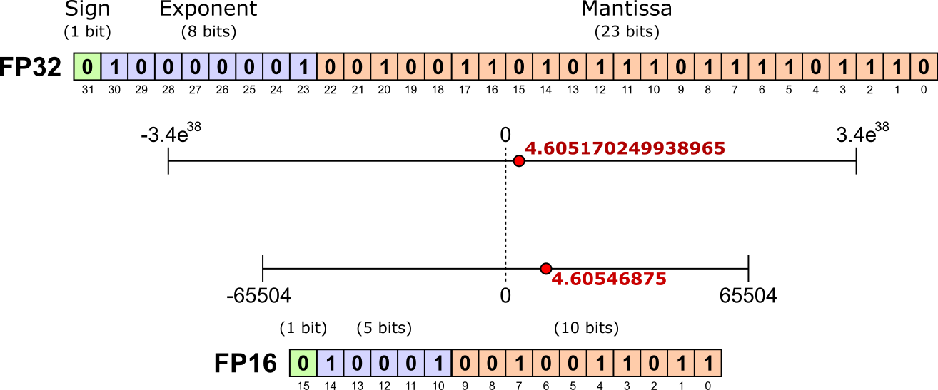
The reduced range and precision poses challenges when working with neural networks. During training, gradients and parameter updates can be extremely small, causing underflow, while activations or intermediate calculations can become large enough to overflow. For this reason, FP16 is often used with mixed-precision training, where most computations use FP16 for speed and memory savings, while sensitive operations — such as gradient accumulation or parameter updates — use FP32. BF16 is often preferred when available because it has a much larger range, similar to FP32, although it provides less precision than FP16.
BF16, or bfloat16, is a 16-bit floating-point format designed primarily for machine-learning workloads. It uses $1$ sign bit, $8$ exponent bits, and $7$ fraction (mantissa) bits. The exponent uses a bias of 127, just like FP32. Because BF16 has the same exponent width as FP32, it supports the same large numerical range from about $-3.4\times 10^{38}$ to about $3.4\times 10^{38}$. However, it has only $7$ fraction bits compared with FP32's 23, providing only a much smaller precision. For example, when representing $\ln{100}$ using BF16, the actual value is $4.59375$.
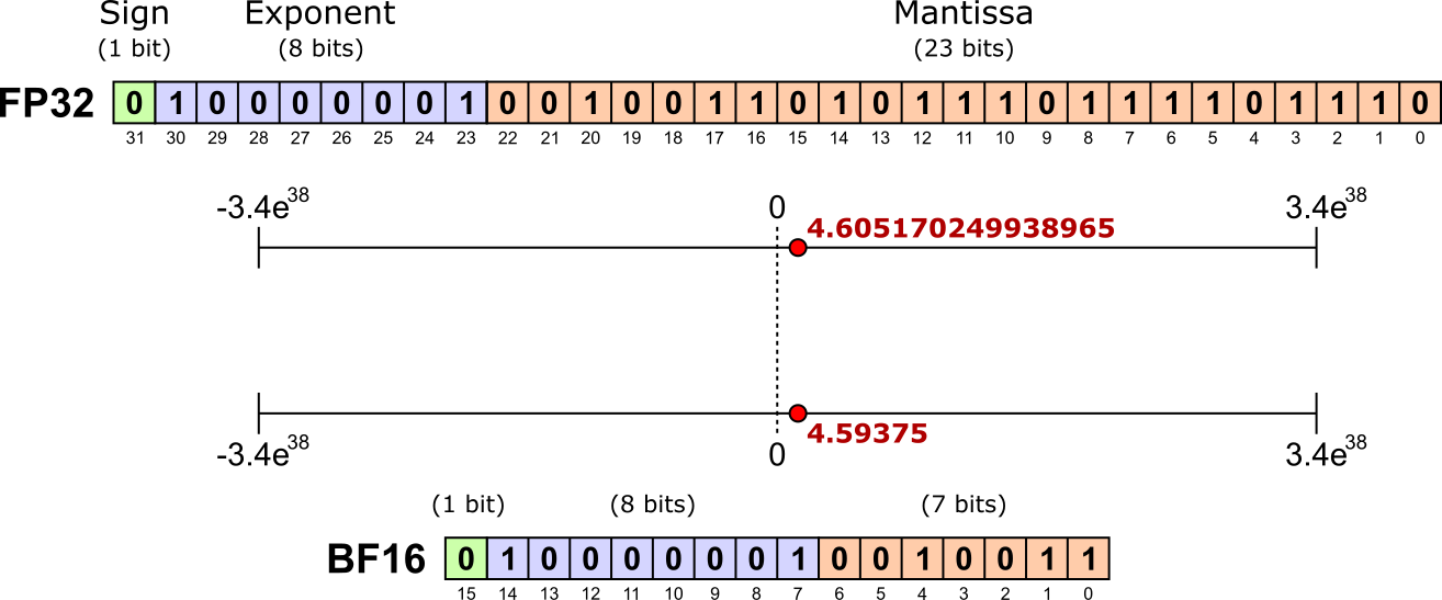
BF16 is often preferred over FP16 because it uses $8$ exponent bits, the same as FP32, and therefore has a similarly large numerical range. This greatly reduces the risk of overflow and underflow when storing activations, gradients, and parameter updates. FP16 has only $5$ exponent bits, so it is more likely to represent very large values as infinity or very small values as zero during neural-network training. BF16 achieves this larger range by using only $7$ fraction bits, so it has lower precision than FP16's $10$ fraction bits. In practice, neural networks are often tolerant of this reduced precision, while the improved range makes training more stable and reduces the need for techniques such as loss scaling. When supported by the hardware, BF16 is therefore commonly preferred; FP16 can still be useful on hardware without efficient BF16 support or when its somewhat higher precision is beneficial.
INT8 is an $8$-bit integer representation that stores whole numbers using exactly $8$ bits. It uses two's-complement encoding and can represent values from $-128$ to $127$. The most significant bit contributes to the sign, while the remaining bits determine the value according to the two's-complement rules. For example, $+5$ is represented as 00000101, while $-5$ is represented as 11111011. Unlike floating-point formats, INT8 has no exponent or fractional part, so it cannot directly represent decimal values. Thus, if we would try to represent $\ln{100}$ using INT8, the actually value would be $4$; note that this might depend on the actual implementation when bits are just cut off (yielding $4$) or if rounding is first applied (yielding $5$).
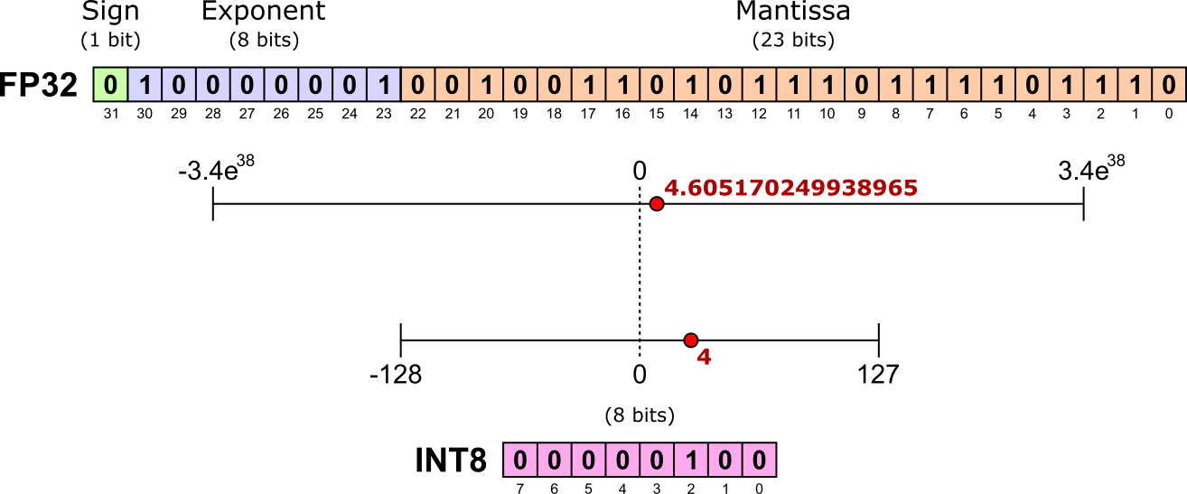
INT8 is generally unsuitable for training neural networks because training requires representing small gradients, parameter updates, and intermediate values with sufficient precision and range. Since INT8 stores only whole numbers between $-128$ and $127$, many small values would be rounded heavily or become zero, making gradient-based optimization unstable or ineffective.
However, a trained model can often be quantized from FP32 or FP16 to INT8 for inference. Quantization maps floating-point weights and activations to INT8 values using scaling factors and sometimes zero points. This reduces memory usage and can significantly improve inference speed and energy efficiency, although the approximation introduced by quantization may cause a small loss in model accuracy. When covering various quantization strategies later, all examples will in fact consider the use case where we want to map numerical values from FP32 to INT8 to reduce the memory footprint of a trained model for inference.
Hands-on: Data Types in PyTorch
To see the use of different data types in action, let's consider PyTorch tensors — although we limit ourselves to $2$-dimensional tensors (i.e., matrices) for a straightforward visualization. In the code cell below, we create a $5\times 4$ tensor with random values sampled from a normal distribution with a mean of $\mu=0$, and a standard deviation $\sigma=5$, i.e., $\mathcal{N}(0,25)$. As motivated at the beginning, weight matrices are explicitly engineered to start normal and tend to stay roughly normal due to initialization choices, loss regularization, and optimization dynamics. The choice of $\sigma=5$ and the random seed (see code cell) below is purely for convenience so that all values have a good spread and stay within the range of $-10$ and $+10$. Lastly, we "manually" set the first (i.e., top-left) entry in the tensor to $\ln{100}$ to have the value we used in the figures above.
# Set random see for consistent outputs
torch.manual_seed(111)
# Specify standard deviation
std = 5
# Create tensor with specific data type
X_fp32 = torch.randn(5, 4, dtype=torch.float32) * std
# Set first value to ln(100)
X_fp32[0][0] = np.log(100)
Since printing the raw tensor using print(X_fp32) does not look very nice — but it is working, of course — we provide the auxiliary method draw_matrix() render vectors and matrices in a more visually pleasing manner. Let's use this method to see how our random FP32 tensor looks like.
draw_matrix(X_fp32)
Although the individual values are not meaningful, we can see how the many shown decimal places reflect the high precision of FP32; and, of course, the first entry representing $\ln{100}$ is the same as shown on the previous figures.
No, let's consider FP16. However, instead of creating a new tensor, we can create a FP16 tensor by casting our FP32 tensor to FP16 using the built-in to() method and passing the torch.float16 data type as argument. This ensures that this new tensor contains the same values, just with reduced precision — also with a reduced range, but since we only have value between $-10$ and $+10$ this does not matter (recall that FP16 has a range from $-65,504$ and $+65,504$). After creating this new FP16 tensor via casting, we can also visualize using the draw_matrix() method.
X_fp16 = X_fp32.to(torch.float16)

draw_matrix(X_fp16)
In simple terms, as we can clearly see, the reduced precision of FP16 means that we no longer have the same amount of decimal places we saw with FP32.
For BF16, we can use the same steps, i.e., casting our FP32 tensor to an BF16 one using the to() method but now passing the torch.bfloat16 data types as argument; and the visualize the resulting BF 16 tensor.
X_bf16 = X_fp32.to(torch.bfloat16)

draw_matrix(X_bf16)
Once again, we see the expected further reduction in precision since BF16 has less mantissa bits than FP16. Thus, just by comparing these to the result here, it seems that FP16 might be the preferred choice. However, you need to remember the BF16 allocates the "missing" bits from the mantissae to the exponent giving it the same numerical range as FP32. It turns out that this tradeoff is often favorable when training neural networks. After all, the whole underlying assumption of quantization is that models are typically overparameterized and we can often live with a reduced precision.
Lastly, we perform the same steps to cast our FP32 tensor to INT8 (i.e., torch.int8).
X_int8 = X_fp32.to(torch.int8)

draw_matrix(X_int8)
As expected our $2$-dimensional tensor now contains only integer values. Once again, particularly by comparing the first entry representing $\ln{100}$, the casting is done by simply "removing" the exponent resulting in the decimal places being cut off. This is $4.6...$ is cast to $4$ instead of $5$ is rounding would do.
Apart from FP32, FP16, BF16, anf INT8, PyTorch supports a wide range of other data types; you can check out the documentation for more details. However, some of the listed data types are so-called shell data types. A shell data type in PyTorch is a lightweight torch.dtype definition designed to act as a container specifier for low-precision and sub-byte formats (e.g., such as FP8, FP4, or INT4) without requiring full native PyTorch C++ kernel implementations for standard operations. These are optimized for special hardware and will not work on any hardware. For example, the code cell below shows how to cast our FP32 tensor to INT4 tensor (i.e., torch.int4), which is likely to fail on your "standard" hardware — but you can give it a shot.
#print(torch.int4)  <-- this line does not yield an error

#X_int4 = X_fp32.to(torch.int4)

#draw_matrix(X_int4)
Of course, reducing precision also means the loss of some information. The advantage is that we need less bits/bytes to store a tensor. In the code cell below, we print for each tensor we have just created the total number of elements using the built-in method numel() — which is of course the same value for all four tensors — the size of each entry in bytes using the built-in method element_size(), as well as the total size of the tensor in bytes (which is simply the product of the two previous values).
for X in [X_fp32, X_fp16, X_bf16, X_int8]:
    print (f"Number of entries: {X.numel()}; size per entry (bytes): {X.element_size()}, total size of tensor (bytes): {X.numel()*X.element_size()}")
Number of entries: 20; size per entry (bytes): 4, total size of tensor (bytes): 80
Number of entries: 20; size per entry (bytes): 2, total size of tensor (bytes): 40
Number of entries: 20; size per entry (bytes): 2, total size of tensor (bytes): 40
Number of entries: 20; size per entry (bytes): 1, total size of tensor (bytes): 20
Side note: Apart from the actual entries, a tensor also requires metadata, including its shape, strides, data type, device, storage location, and a reference to the underlying memory. If automatic differentiation is enabled, additional memory may be required for gradients and the computation graph. The actual memory footprint can therefore be larger than the data payload alone. On GPUs, memory allocation may introduce further overhead due to alignment, allocator bookkeeping, and PyTorch's caching allocator, which may reserve more memory than the tensor currently uses. Furthermore, tensor views can share the same underlying storage, meaning that several tensors may have separate metadata but not separate data buffers. Distinguishing between raw data size, tensor-object overhead, and reserved device memory is therefore important when analyzing and optimizing memory usage but way beyond our scope here.
In some sense, downcasting a tensor to a lower-precision data type can already be considered a form of quantization. After all, we have reduced the required memory in exchange for some loss of information (i.e., reduced precision). However, as we will see later, this would be a very naive approach for a quantization strategy as the loss of information we have is unnecessarily high. Proper strategies can do much better.
Before looking into proper quantization strategies next, let's briefly implement an auxiliary method we will be using later to actually implement quantization from scratch. The method get_dtype_bits() takes in a Pytorch data type and returns the amount of bits required to store a value of this data type. get_dtype_bits() is simply a wrapper for the built-in PytTorch methods torch.iinfo() and torch.finfo(). The former information about an integer data type (e.g., torch.int8, torch.int32, torch.int64); the latter serves the same purpose for floating-point data types (e.g., torch.float16, torch.float32, torch.float64). Both their return objects have the attribute bits to get the number of required bits.
def get_dtype_bits(dtype):
    try:
        return torch.iinfo(dtype).bits
    except Exception as e:
        return torch.finfo(dtype).bits
For a quick test, the code cell below used this method to get the number of bits we need to store a value for the data types we have considered so far FP32 (torch.float32), FP16 (torch.float16), BF16 (torch.bfloat16), and INT8 (torch.int8).
print(f"Number of bits to store FP32:  {get_dtype_bits(torch.float32)}")
print(f"Number of bits to store FP16:  {get_dtype_bits(torch.float16)}")
print(f"Number of bits to store BF16:  {get_dtype_bits(torch.bfloat16)}")
print(f"Number of bits to store INT8:  {get_dtype_bits(torch.int8)}")
Number of bits to store FP32:  32
Number of bits to store FP16:  16
Number of bits to store BF16:  16
Number of bits to store INT8:  8
The get_dtype_bits() method will later help when we want to quantize a tensor into some target data type we specify.
Basic Quantization Strategies
The core idea of quantization is to convert high-precision but memory-demanding data into lower-precision but memory-saving data. The motivation is that, particularly in the context of working with large and often over-parameterized neural networks, lower precision often does not negatively affect the model performance (much); and we can use much more efficient use of the expensive and often limited resource of memory (particularly VRAM). We just saw that, at least in principle, we can already achieve this by down-casting, say, an FP32 tensor to an INT8 tensor of roughly only quarter the original size. However, the loss of information of this naive approach is unnecessarily high for multiple reasons — we use the casting of FP32 to INT8 tensor as an example:
No rescaling: Casting an FP32 value directly to INT8 typically removes just its fractional part and stores the remaining integer. However, it does not rescale the values to use INT8's full range of $−128$ to $127$. Consequently, many similar FP32 values can map to the same INT8 value (for example, $3.1$, $3.7$, and $3.99$ may all become $3$) causing significant precision loss. Rescaling the values to the full range of the target data type (here: INT8) reduced this risk, even if it cannot be completely avoided.
Out-of-range values: INT8 can represent only integer values from $−128$ to $127$, while FP32 supports a much larger range. Therefore, casting an FP32 value outside the INT8 range can cause overflow, truncation, or wraparound, depending on the operation and backend. For example, converting $200.0$ to INT8 cannot represent the original value. It may produce an unexpected result such as $-56$ due to wraparound rather than a meaningful approximation.
In the section, where we cover the two most basic quantization strategies — asymmetric quantization and symmetric quantization we address the rescaling issue . In the following section, where we consider the effect of outliers, we address out-of-range values.
For all examples shown below, we will be using our $5\times 4$ tensor X_fp32. Recall that its $20$ values have been sampled from a normal distribution $\mathcal{N}(0,25)$. Recall that weights in a neural network are often initialized using a zero-centered normal or similar distribution. During training, they frequently remain approximately centered around zero because positive and negative values are useful for balancing signals, while optimization and regularization tend to prevent extreme values. Although not guaranteed, trained weights often roughly retain their normal distribution. The figure below illustrates this idea by plott the distribution of the values X_fp32 tensor; due to limited space, it only shows the minimum and maximum weight — keep in mind that $20$ values are generally not enough to properly "see" the normal distribution in the data.
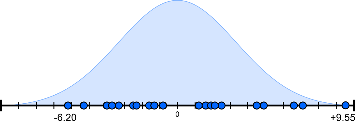
Let's now see how quantization works using X_fp32 with its $20$ weights as an example input. However, to ease presentation and show exact numbers, we only consider $10$ of the $20$ weights rounded to $1$ decimal place as shown below. Since we quantize to INT8 all examples, the exact FP32 values in the original tensor are not important.

In general, quantization aims to preserve the original distribution as closely as possible. This is important because the distribution of these values influences the computations throughout the neural network. Excessive distortion can change the outputs of individual layers and accumulate into a significant loss of model accuracy. For this reason, quantization commonly uses a linear mapping between the input and output ranges. The input values are scaled (and, if needed, shifted using a zero-point) so that their relative distances are approximately preserved in the lower-precision representation. So let's see how this works.
Asymmetric Quantization
Recall that we want to utilize the numerical range of the lower-precision data as much as possible to minimize the risk that two FP32 values get mapped to the same INT8 to preserve as much information as possible. Asymmetric quantization accomplishes this by mapping the smallest weight (here: $-6.2$) to the minimum INT8 value $-128$, and the largest weight (here: $9.6$) to the maximum INT8 value $128$. For this mapping we need to scale and shift the FP32 values such that they occupy the INT8. For the scaling, we compute the scaling factor $s$ as:
where $\text{max}(\mathbf{X})$ and $\text{min}(\mathbf{X})$ return the largest and smallest weights of tensor $\mathbf{X}$; $b$ is the number of bits for the lower-precision data type (here: $b=8$ for INT8). For example, using the smallest and largest weights from our tensor X_fp32, we get the following value for the scaling factor:
We can then compute the zero-point $z$ telling us how much we need to shift the scaled values using:
Again, to show an example, plugging in all the values for our example tensors, we get:
With the scaling factor $s$ and the zero-point $z$, we can quantize and the input tensors $\mathbf{X}$ from to get is quantized version $\mathbf{X}_{quant}$, but the also dequantize it to get $\mathbf{X}_{quant}$ reflecting the corresponding mapping from the lower-precision space to the high-precision space; the two respective expression are:
We can now use the first expression to quantize your example tensor X_fp32 to INT8 using the scaling factor $s=16.1$ and zero-point $z=-28$. The figure below illustrates this mapping from FP32 to INT8. Note that the size of the ranges are not to scale; while the actual weight values are between $-10$ and $+10$, the figure aims to reflect that the numerical range of FP32 is (much) larger than the one of INT8. We can clearly see how the smallest and largest weight maps to the minimum and maximum value that can be represented by INT8. All values between the smallest and largest weight map into to range of INT8, roughly preserving the original distribution.
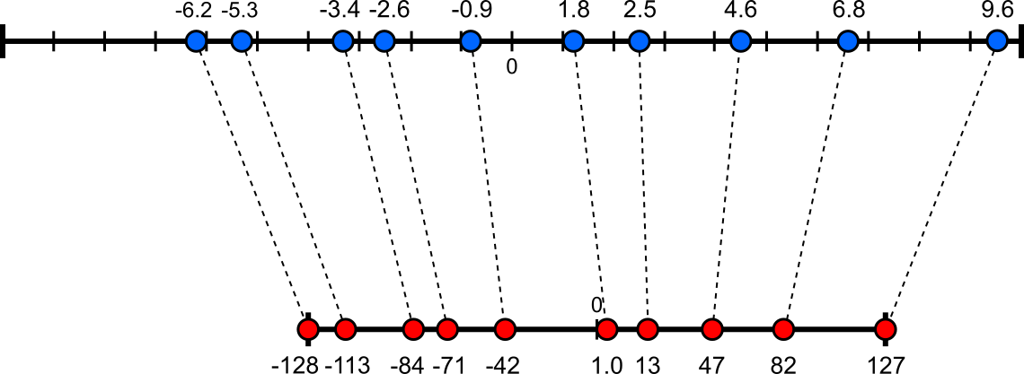
Notice how the $0$ is shifted; in our example, the FP32 value $0.0$ maps to the INT8 value of $-28$ (i.e., the value for $z$). This is simply because the smallest and largest weights do not have the same distance in the FP32 space, but then they do in the INT8 space. Before discussing the pros and cons of asymmetric quantization, let's first have a look at symmatrix quantization to allow for a direct comparison.
Symmetric Quantization
In simple terms, symmetric quantization maps $0.0$ in the FP32 space to $0$ in the INT8 space — recall that we consider the quantization of an FP32 tensor to an INT8 tensor as an example, but the overall idea remains the same. We can easily accomplish this by first finding the absolute maximum value in the original tensor $\mathbf{X}$; let's call it $alpha$ and which can be computed as:
For our example tensor X_fp32 we already know that $\text{min}(\mathbf{X}) = -6.2$ and $\text{max}(\mathbf{X}) = 9.6$, giving us a maximum absolute value of $\alpha = 9.6$. We can now use $-\alpha$ and $+\alpha$ as the lower and upper bound to compute our scaling factor $s$:
If we use the number from example tensor X_fp32, we get:
Since we enforce that FP32 $0.0$ maps to INT8 $0$, we do not need any zero-point for correction. However, we can convince ourselves that this is indeed the case by computing zero-point $z$ for our example and symmetric quantization:
With $z=0$, the expressions for quantizing a tensor $\mathbf{X}$ to get $\mathbf{X}_{quant}$ and to dequantize it back to get $\mathbf{X}_{dequant}$ simplify to:
Like before, we can visualize symmetric quantization for our concrete example to show how each original FP32 weight in tensor X_fp32 maps to its corresponding value in the INT8 space; see the figure below. Naturally, not the smallest original weight no longer maps to $-128$, i.e., the smallest possible value of the numerical range of INT8.
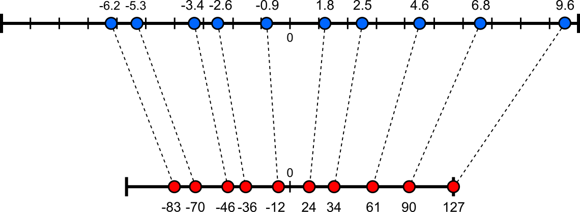
In short, asymmetric and symmetric quantization are very similar. The only difference is which values for the lower and upper bound in the denominator of the expression for computing the scaling factor $s$.
Implementation & Examples
We just saw that all expressions required for quantization, both asymmetric and symmetric quantization, are quite straightforward. This also means that they can easily be implemented. So let's look and test a basic toy implementation for quantizing and dequantizing a PyTorch tensors. To this end, the method get_scale_and_zeropoint() in the code cell below computes the scaling factor s and the zero-point $z$ for a given input tensor X by performing the following main steps:
- Extract the smallest and largest value in input tensor
X - Identify the value of $b$ depending on the target data type using the auxiliary method
get_dtype_bits() - Compute $s$ and $z$ depending on whether asymmetric or symmetric quantization is performed (in case of symmetric quantization, we first need to compute the absolute maximum)
def get_scale_and_zeropoint(X, quant_type=torch.int8, symmetric=False):
    # Fing the smallest and largest value in tensor X
    x_min = torch.min(X).item()
    x_max = torch.max(X).item()
    # Get range of target data type for quantization (i.e., b = number of bits)
    b = get_dtype_bits(quant_type)
    # Check if symmetric quantization is specified
    if symmetric == False:
        # Cpmpute scaling factor and zero-point
        s = (2**b - 1 ) / (x_max - x_min)
        z = -np.round(x_min * s) - 2**(b-1)
    else:
        # Compute absolute maximum
        alpha = np.max((np.abs(x_min), np.abs(x_max)))
        # Compute scaling factor; we know z=0
        s = (2**b - 1 ) / (2*alpha)
        z = 0.0
    # Return scale and zero-point
    return s, z
We can test the method by applying it to our example tensor X_fp32 to get the scaling factor $s$ and zero-point $z$. Of course, apart from precision issues, the result matches the one we calculated directly in the examples above. First, we consider asymmetric quantization.
scale, zero_point = get_scale_and_zeropoint(X_fp32, symmetric=False)

print(f"Asymmetric Quantization")
print(f"Scale factor: {scale:.5f}")
print(f"Zero-point: {zero_point:.5f}")
Asymmetric Quantization
Scale factor: 16.19171
Zero-point: -28.00000
Now we can do the same for symmetric quantization by simply setting symmatric=True when calling the method.
scale, zero_point = get_scale_and_zeropoint(X_fp32, symmetric=True)

print(f"Symmetric Quantization")
print(f"Scale factor: {scale:.5f}")
print(f"Zero-point: {zero_point:.5f}")
Symmetric Quantization
Scale factor: 13.34927
Zero-point: 0.00000
Having computed the scaling factor and the zero-point, we can implement the simple expressions we have that quantize and dequantize a tensor; see the code cell above for example implementations. Given the simplicity of the two expressions, the code might look unnecessarily complex, this has to main reasons:
In both the
quantize()anddequantize()method, we explicitly distinguish between asymmetric quantization ($z\neq0$) and symmetric quantization ($z=0$). Although adding or subtracting a zero-point of $0$ does not change the result, simply performing the computations can have a noticeable effect on the compute on a large scale. Thus if we can avoid it in case of symmetric quantization, then we should.In the
quantize()method we first identify the minimum and maximum possible value that can be expressed using the target data type. This is to ensure that after the mapping from the high-precision space to the lower-precision space the values do not roll over. For example, due to the rounding, the largest FP32 weight might map to128. However the maximum possible INT8 value is127. When casting128to INT8, it would roll over and become $-128$. To avoid this, we clamp the mapped values that none of them is outside the allowed range.
def quantize(X, scale, zero_point, quant_type=torch.int8):
    # Get minimum and maximum possible value for quant_type
    try:
        dtype_info = torch.iinfo(quant_type)
    except Exception as e:
        dtype_info = torch.finfo(quant_type)
    q_min, q_max = dtype_info.min, dtype_info.max
    # Quantize and clamp tensor (to avoid "rollover") issues
    if zero_point == 0.0:
        return torch.clamp(torch.round(X*scale), q_min, q_max).to(quant_type)
    else:
        return torch.clamp(torch.round(X*scale) + zero_point, q_min, q_max).to(quant_type)

def dequantize(X, scale, zero_point, quant_type=torch.float32):
    # Dequantize and return tensor
    if zero_point == 0.0:
        return (X / scale).to(quant_type)
    else:
        return ((X - zero_point) / scale).to(quant_type)
We are finally ready to properly quantize our example tensor X_fp32 to INT8 (the default target data type, but you can change that for testing). In the code cells below, we only consider asymmetric quantization as showing both cases does not provide additional insights. However, you can also try symmetric quantization by setting symmatric=True. After quantization, we visualize both the input tensor and the quantized tensor for a direct comparison.
# Compute scaling factor and zero-point
scale, zero_point = get_scale_and_zeropoint(X_fp32, symmetric=False)

# Quantize input tensor
X_quant = quantize(X_fp32, scale, zero_point)

print(f"Original tensor:")
draw_matrix(X_fp32)
print(f"\nQuantized tensor:")
draw_matrix(X_quant)
Original tensor:
Quantized tensor:
In case of asymmetric quantization, as expected, we can see that the quantized tensor contains both the minimum ($-128$) and the maximum ($127$) possible value of INT8.
Lastly, the interesting part is when we dequantize the quantized tensor, i.e., in our example, dequantize the INT8 tensor back to FP32. For this, we only call the dequentize() method on the quantized tensor X_quant and visualize the resulting dequantized tensor.
# Dequantize tensor
X_dequant = dequantize(X_quant, scale, zero_point)

print(f"Dequantized tensor:")
draw_matrix(X_dequant)
Dequantized tensor:
When compared with the original FP32 tensor, the dequantized tensor looks indeed very similar. To get some better insights, we can compute the quantization error as the difference between each corresponding tensor entry in the original and the dequantized tensor. This difference is, of course, just another tensor which we can display as shown in the code cell below.
# Compute error as difference between original tensor and dequantized tensor
X_error = X_fp32 - X_dequant

print(f"Quantization error (elementwise):")
draw_matrix(X_error, decimals=5)
Quantization error (elementwise):
As expected, quantization generally leads to a loss of information, meaning that we cannot reconstruct the original FP32 tensor from its quantized version. On the other hand, when comparing the original values with the elementwise error, we can see that the errors are arguably rather small. We can see this even better when computing the elementwise error as percentage as shown below.
X_error_percent = np.round(X_error * 100 / X_fp32, decimals=2)

print(f"Quantization error (elementwise, percentage):")
draw_matrix(X_error_percent, decimals=2)
Quantization error (elementwise, percentage):
As we can see, all errors remain, in absolute terms, below 3% and in most cases below 1% compared to the original values. In the context of over-parametersized neural networks, this loss of information often does not result in any significant degradation of the models performance but comes with a significant decrease in its over memory footprint.
Discussion
In terms of their required calculation and therefore also their implementation, asymmetric and symmetric quantization are fundamentally very similar. However, regarding their application in practice, both quantization strategies have their pros and cons that may recommend one strategy over the other depending on the exact situation. On a high level, the two considerations are:
Bit utilization. Asymmetric quantization always makes full use of the numerical range of the lower-precision data type. This maximizes the spread of the mapped values and thus minimizes the loss of information. In contrast, symmetric quantization may under-utilize the numerical range particularly if the distribution of the original values are (very) skewed. This increases the risk that two values that are different in the original space will map to the same value in the target space. Overall, this means a greater loss of information.
Performance. Asymmetric typically involves a non-zero zero-point ($z\neq0$) that needs to be added or subtracted during the quantization or dequantization steps. While subtracting an integer seems trivial at the scalar level, in high-performance matrix multiplication, non-zero zero-points fundamentally disrupt how hardware accelerators maximize throughput. On dense, massively parallel accelerators (GPUs/TPUs/NPUs), this can translate to a noticeable 15% to 30% execution latency penalty. Of course, symmetric quantization with $z=0$ does not have this issue.
In short, choosing between asymmetric and symmetric quantization involves a tradeoff between minimizing information loss and maximizing computational performance. Asymmetric quantization often reduces quantization error but introduces additional correction terms during integer arithmetic. Symmetric quantization uses a simpler zero-centered mapping, which generally leads to more efficient and easier-to-optimize hardware operations but potentially causes greater information loss.
In practice, the choice between asymmetric and symmetric comes down "where" the strategy is applied. Asymmetric quantization is typically favored when we have to deal with non-zeroed distributions or aim for a really low-bit quantization. The table below outlines most common situations where asymmetric quantization is likely to be the preferred choice.
| Situation | Rationale |
|---|---|
| One-sided activations, such as ReLU, GELU, and SiLU | Values are often non-negative. Asymmetric quantization uses the integer range more effectively instead of reserving half of it for negative values. |
| Ultra-low-bit quantization, such as INT4 or INT3 | Wasting part of the available range is especially costly at low bit widths. Asymmetric quantization preserves more quantization levels and reduces accuracy loss. |
| LLM KV-cache compression | Key-value caches can have directional biases or non-zero-centered ranges. Asymmetric quantization can preserve attention quality more effectively. |
In contrast, we generally prefer symmetric quantization when we do not require the benefits of asymmetric quantization to maximize performance — or when performance is very critical and we can or have to live with a potentially higher quantization error. Again, the table below outlines common situations for that.
| Situation | Rationale |
|---|---|
| Model weights | Weight distributions are often approximately Gaussian and centered around zero, making a zero-point of zero suitable. |
| Latency-critical edge devices | Microcontrollers, DSPs, and AI chips benefit from simpler zero-point-free integer arithmetic and optimized fast paths. |
| Zero-centered activations, such as Tanh or identity outputs | Symmetric quantization matches distributions containing both positive and negative values centered around zero. |
To sum up, despite their close relationship, asymmetric and symmetric do have different characteristics that do matter in practice.
Handling Extreme Values
So far, we have assumed that the distribution of values before quantization is reasonably well-behaved, even if it is skewed and/or not zero-centered. This particularly means that the input values do not contain any extreme values, i.e., values very far away from the mean (e.g., the mean of values in a weight matrix or the mean of activations of a layer). However, even with optimal Gaussian initialization, extreme values (outliers) inevitably emerge during training as the network scales, learns highly specialized representations, and optimizes against unconstrained loss objectives. For example, weight outliers may occur due to:
- Cross-Entropy loss dynamics: Softmax classification loss drives predicted probabilities toward $1.0$, which mathematically requires driving target logit values toward infinity. To achieve higher prediction confidence, gradient updates continually inflate the weight vector magnitudes in final and penultimate layers.
- Rare feature specialization: Neurons assigned to detect highly specific, low-frequency patterns (e.g., rare vocabulary words or niche visual features) receive sparse but massive gradient spikes. Over millions of steps, these specific weight parameters expand disproportionately to trigger strongly when that rare pattern occurs.
- Unregularized parameters: Modern training pipelines often exclude specific parameter groups (such as bias terms, LayerNorm scales $\gamma$, or positional embeddings) from L2 weight decay. Unbounded by regularization penalties, these specific weight matrices can drift to extreme dynamic ranges over time.
When it comes to activations, particularly in the context of Transformer-based LLMs, outliers may occur due to:
- Unbounded activation functions: Non-linearities like ReLU, GELU, and SiLU have no upper limit ($[0, \infty)$). When strong input signals align across multiple layers, pre-activations pass through unchecked into very large scalar values.
- Residual stream accumulation: Architectures using residual connections ($x + f(x)$) continuously add transformed outputs back into the main signal path. Across dozens or hundreds of stacked layers, this additive stream naturally compounds activation variance and peak magnitudes.
- Softmax sharpness in attention: To generate focused attention heads, the model must feed large scalar inputs into the $\text{Softmax}$ function to make the exponentiated values approach $1.0$ for target tokens while driving others toward $0.0$.
In short, extreme values in the distributions of weights or activations are not rare cases but are a rather common occurrence.
What Can Go Wrong?
To see how extreme values can negatively affect quantization, let's first use our implementation to run an example. To this end, the code cell below creates a copy of our initial example tensor X_fp32 but then changes the bottom left entry to an extreme value. The default value of $-333.3$ was chosen to be large enough to clearly see the change in the quantized tensor and the quantization errors but not too large for everything to "collapse". However, you are encouraged to change this value of that outlier see how it affects all following outputs.
X_fp32_outlier = X_fp32.clone()

X_fp32_outlier[-1][0] = -13.3

draw_matrix(X_fp32_outlier)
We now quantize this new FP tensor to INT8 as seen before. Again, we go with asymmetric quantization by default, but in case of extreme values this does not really make a difference. Still, feel free to switch to symmetric=True to perform symmetric quantizations.
# Compute scaling factor and zero-point
scale, zero_point = get_scale_and_zeropoint(X_fp32_outlier, symmetric=True)

# Quantize input tensor
X_quant = quantize(X_fp32_outlier, scale, zero_point)

print("\nQuantized tensor (with outlier):")
draw_matrix(X_quant)
Quantized tensor (with outlier):
Just by looking at the output, you should already see the issue. As the outlier is negative, it gets mapped to the minimum INT8 value $-128$. However, since asymmetric (but also symmetric) quantization is a linear mapping to preserve the input distribution as much as possible, all other values gets mapped to the the very upper end of the numerical range if INT8. In fact, the quantized tensor now contains several subsets of values of the same value — in other words, different FP32 values have collapsed to the same INT8 value, which did not happen without that extreme value (see above).
To really see the issue, the code cell below dequantized the quantized tensor and computes the relative error percent for each entry.
# Dequantize tensor
X_dequant = dequantize(X_quant, scale, zero_point)

# Compute error as difference between original tensor and dequantized tensor
X_error = X_fp32_outlier - X_dequant

# Compute relative error in percent
X_error_percent = np.round(X_error * 100 / X_fp32, decimals=2)

print(f"Quantization error (elementwise, percentage):")
draw_matrix(X_error_percent, decimals=2)
Quantization error (elementwise, percentage):
Now the relative errors are much higher compared to the ones we saw before (without having an extreme value in the input tensor). This simply means that the information loss is now much greater and the model performance is very likely going to degrade because of this.
We can also illustrate the effects of extreme values using the same visualization as before. While not to scale, the figure below now shows the mapping from the FP32 values including the outlier — assuming the default values of $-333.3$ — to their corresponding INT8 values between $-128$ and $127$ when performing asymmetric quantization.
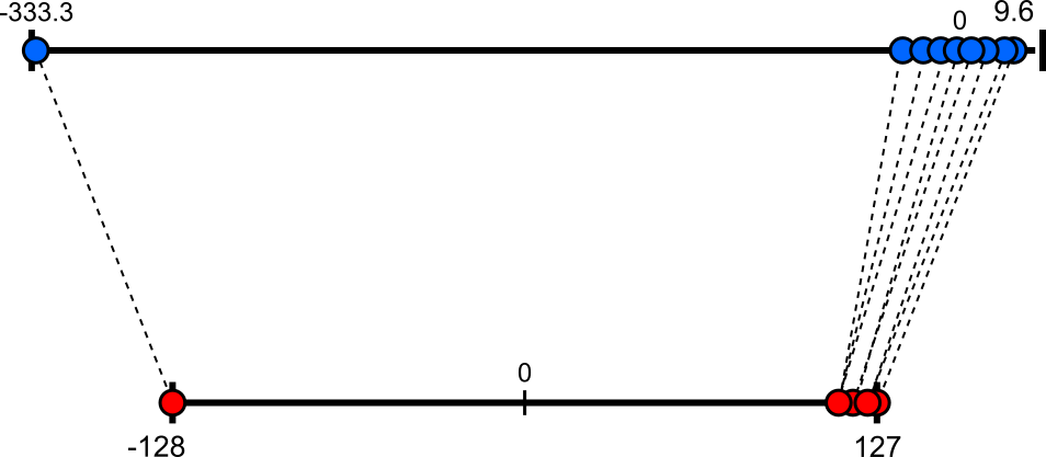
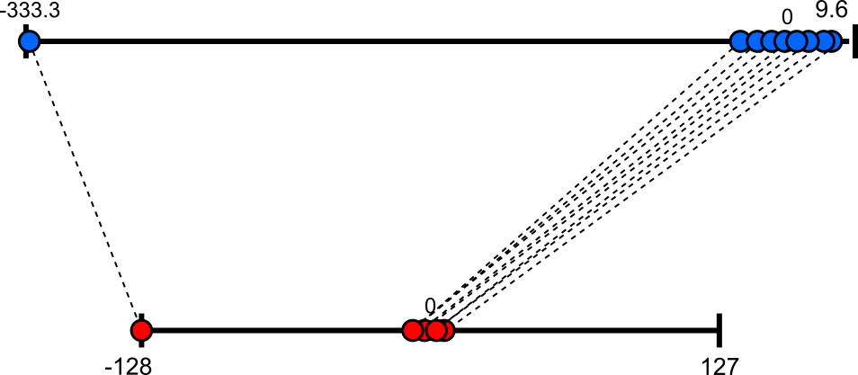
For the sake of completeness, the figure below shows the corresponding result when performing symmetric quantization instead of asymmetric quantization. Here, all remaining values are now tightly clustered around $0$. In fact, they are more tightly clustered compared to asymmetric quantization because, recall, asymmetric quantization has a better bit utilization and spread all values across the whole numerical range of the target space (here: INT8).
In short, not only can extreme values (outliers) commonly occur in the distributions of weights and activations, they also can have a significant negative effect on the quantization results, yielding an unacceptable loss of information through quantization. Thus, to avoid performance degradation of the model, extreme values need to be handled in practice.
Clipping
Now that we know the problems that extreme value can cause, the solution is — at least at a first glance — quite straightforward: clipping (or clamping), which limits values to a predefined range before quantization. Values below the lower bound are replaced by the lower bound, while values above the upper bound are replaced by the upper bound. Clipping prevents a few extreme outliers from determining the quantization scale and consuming a large portion of the available integer range. This improves the precision for the majority of values, but also poses its own challenges, as we will see in the moment.
First, let's go through a complete example using our example tensor containing that one extreme value. Clipping a tensor is in fact very easy since PyTorch provides the built-in method clip() for that. Apart from the input tensor, we can also specify the lower and upper bound. In the code cell below, we set the lower bound to $-10$ and the upper bound to $+10$ — mainly because for this example we know that those are good bounds — but you can play with both bounds to see how the results change. After clipping, we simply display the resulting tensor.
X_fp32_clipped = torch.clip(X_fp32_outlier, -10, 10)

draw_matrix(X_fp32_clipped)
Notice how the extreme values $-333.3$ (assuming the default value) of the bottom-left entry has changed to $-10$ as expected. Let's now quantize this clipped tensor like we did before.
# Compute scaling factor and zero-point
scale, zero_point = get_scale_and_zeropoint(X_fp32_clipped, symmetric=True)

# Quantize input tensor
X_quant = quantize(X_fp32_clipped, scale, zero_point)

print("\nQuantized tensor (after clipping):")
draw_matrix(X_quant)
Quantized tensor (after clipping):
Of course, the former extreme value now clipped to $-10$ still maps to $-128$, the minimum possible values of the numerical range of INT8. However, all remaining values are no longer clumped together near the upper end of the range but again much more spread apart, very similar to originally quantized tensor without the extreme value. We can confirm this by once again dequantizing the vector and compute the quantization errors for each entry in the tensor.
# Dequantize tensor
X_dequant = dequantize(X_quant, scale, zero_point)

# Compute error as difference between original tensor and dequantized tensor
X_error = X_fp32_outlier - X_dequant

# Compute relative error in percent
X_error_percent = np.round(X_error * 100 / X_fp32, decimals=2)

print(f"\nQuantization error (elementwise, percentage):")
draw_matrix(X_error_percent, decimals=2)
Quantization error (elementwise, percentage):
The output above makes it very clear: While the relative errors of the non-outlier values are close to the original errors for the tensor without the extreme value, the error for the outlier itself is not very large. This is the quantized value reflecting the extreme value that gets naturally dequantized to around $-10$ (i.e., the lower clipping bound). This value is of course very different from the true value of $-333.3$ before the clipping, resulting in this huge relative error. This means that clipping involves balancing two competing sources of distortion:
- Clipping error (saturation): information loss due to extreme outliers being "crushed" into the maximum boundary; this includes that all values beyond the boundaries get clipped to the same boundary value and therefore become indistinguishable (note that in our simple example, we had only one tensor entry outside the clipping boundaries).
- Quantization error (rounding): precision loss because the step size between adjacent integer bins is too wide; in this case, more non-outliers may become indistinguishable because they get mapped to the same value.
In general, setting the clipping threshold (i.e., the boundaries) too wide causes high quantization noise; setting it too narrow causes high clipping distortion. Finding the sweet spot for the clipping threshold is commonly done by the called calibration, which we have to discuss next.
Side note: Clipping can use either symmetric thresholds (e.g., $[-10, +10]$) or asymmetric thresholds (e.g., $[-20, +10]$. The choice of approach is closely related to the choice of the initial quantization strategy. While asymmetric thresholds are more appropriate for skewed or one-sided distributions (e.g., ReLU activations) they may come with a significant performance penalty depending on the underlying hardware. In contrast, while symmetric thresholds simplify the quantization process and integer arithmetic, they assume value distributions centered around $0$ — well, at least for the vast majority of values apart from the one or more extreme values.
Calibration
In the example above motivating the purpose of clipping we "manually" picked the thresholds, i.e., the lower and upper bound for the clipping, to be the range $[-10, +10]$. We could do this because we know how the example tensor was generated, including that the values apart from the outlier were in this range. In practice, of course, this is not straightforward. Even we just consider the final weight matrices of a trained model and assume that the weights in each layer are approximately normally distributed, their scales can differ substantially.
These differences can arise from the layer's fan-in and fan-out (i.e., its input and output size), the scale of its inputs and gradients, normalization layers, architectural structure, and the optimization process. During training, different layers receive different update magnitudes and may require different weight scales to produce useful activations. Regularization may reduce large weights but does not force all layers to share the same variance. This is why quantization often uses separate scaling factors and zero-points for different layers — or even multiply scaling factors and zero-points special types of layers (e.g., individual quantization parameters for each channel in a Convolutional Neural Network (CNN)).
Finding optimal clipping thresholds is non-trivial because neural network performance is exceptionally sensitive to the balance between clipping noise (saturation) and quantization noise (rounding). Finding boundaries that minimize end-to-end task degradation requires solving complex optimization trade-offs, where the practical approach depends on two core dimensions:
When does Quantization Occur? In the simplest case, quantization is performed only post training, i.e., after the model has been fully training using full precision. At this point, the learnable parameters of a model (e.g., weights, basis, activation or normalization layer parameters, etc.) no longer change. Here, finding the best clipping thresholds is mostly an offline search problem using statistical heuristics (e.g., KL-divergence, MSE minimization, or search-based algorithms). In contrast, quantization can be applied during training where all model parameters still change over time. In this case, the clipping thresholds typically become learnable parameters optimized during the training. This approach poses a wide range of challenges to ensure a good model performance
Which Values are Quantized? When using post-training quantization, weights and biases are static and fully known prior to deployment; however, note that biases are typically left in higher precision to prevent systematic output drift. This makes finding good clipping thresholds somewhat more straightforward. In contrast, activations are dynamic and vary with every inference query. Deep models (particularly Transformer architectures) exhibit systemic "activation outliers", i.e., extreme magnitude spikes concentrated in specific feature channels. Static offline thresholds risk aggressively crushing these high-value activations, while dynamic online thresholding (calculating statistics on the fly during inference) introduces latency and memory overhead.
Finding the optimal clipping thresholds — even for the simpler case where quantization is applied only after the training — is far from a straightforward process, and a more detailed discussion about different approaches is beyond the scope of this introductory notebook.
What's Next?
In this notebook, we focused on the following three main questions regarding quantizing neural networks:
- What is the main goal? $\rightarrow$ Reduce the memory footprint of large neural networks, particularly of (Transformer-based) Large Language Models.
- *Why does it work?* $\rightarrow$ Large models are often over-parameterized and use various components and strategies that make them less sensitive to the precision of individual values (weights, biases, activations).
- How does it work? $\rightarrow$ Basic strategies for asymmetric and symmetric quantization, including clipping (with calibration) to handle extreme values.
While we saw quantization in action using an example tensor representing the weight matrix of a network layer, we did not actually cover how quantization is integrated or applied to a full network in practice. This is because there are various approaches to do this, and even the arguably most basic ones pose practical challenges that require a dedicated and detailed discussion. In the following, we therefore provide only a brief overview to the most common approaches for quantizing neural networks.
Post-Training Quantization (PTQ)
Post-Training Quantization (PTQ) converts a fully trained, high-precision floating-point model (such as FP32) into a lower-precision integer format (such as INT8) after training is completely finished, without requiring model retraining. Its primary advantage is operational simplicity: because it bypasses backpropagation, gradient calculations, and complex training pipelines, developers can quantize a neural network in minutes using only a small representative calibration dataset or simple analytical routines.
The mechanics of PTQ are relatively straightforward because of how it standardizes parameter bounds prior to deployment. For one, weights are static after training, so their ranges and distributions can be inspected directly to determine suitable scales, zero-points, and clipping thresholds. Activations, however, are not static but depend on the input data and can vary between samples. PTQ therefore typically uses a representative calibration dataset to observe activation ranges and estimate their quantization parameters — which is still considered relatively straightforward and can be done on an offline stage before actually deploying the model.
However, PTQ has its limitations. Most obviously, PTQ strictly benefits only the inference phase, offering zero memory or computational savings during training since it is applied exclusively after a model is fully trained. Beyond this phase limitation, PTQ's primary drawback is parameter rigidity: because model weights are frozen, they cannot adapt via backpropagation to compensate for the introduced rounding and clipping noise. Consequently, PTQ frequently suffers severe accuracy drops when quantizing to lower bit-widths (e.g., INT4) or when applied to sensitive model architectures. Additionally, PTQ is highly vulnerable to calibration failures and activation outliers. Because activation bounds are set statically during offline calibration, performance relies entirely on how closely the calibration sample mimics real-world data. Any runtime distribution shift forces unseen inputs into suboptimal dynamic ranges, causing heavy clipping distortion or quantization noise.
Post-Training Quantization (QAT)
QAT aims to be less sensitive to outputs not seen during the calibration through training a model using full precision while simulating the effects of quantization. This is typically done through fake-quantization operations. A fake-quantization operation does not usually convert the tensor permanently to an integer during training. Instead, it simulates quantization by scaling, rounding, clipping, and scaling back to floating point, allowing the model to experience quantization effects while remaining trainable. The figure below illustrates the idea of a "fake quant" to simulate the effect of quantizing the activation of one layer before passing the dequantized values to the next layer.
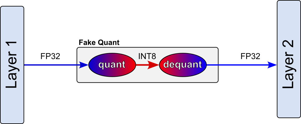
QAT can also generalize better to new inputs because the model learns to operate under quantized conditions rather than being calibrated only after training. However, it does not completely eliminate distribution-shift problems. If new inputs produce activation values outside the ranges encountered during training, clipping can still occur. QAT therefore still requires representative training data and an appropriate strategy for handling activation ranges during inference.
Overall, QAT makes optimization more challenging because the forward pass simulates low-precision inference while the model is trained using high-precision parameters. During this process, activations and weights pass through fake-quantization operations that scale, clip, and round their values. However, rounding and clipping are not differentiable in the usual sense, which makes direct gradient-based optimization difficult. QAT therefore relies on approximations such as the straight-through estimator (STE) to allow gradients to pass through these operations. Even with this approximation, the simulated quantization noise can make training less stable and may require careful choices of learning rate, initialization, calibration, and training duration.
Quantized Training (QT)
Fully Quantized Training (QT) attempts to perform the entire training process using low-precision representations. This can include quantizing weights, activations, gradients, parameter updates, and optimizer states rather than using high-precision master weights and accumulators. The goal is to reduce training memory consumption, data movement, and potentially energy usage, which could make training large models or performing on-device training more efficient.
QT is much more challenging because gradients and parameter updates are often small, highly variable, and sensitive to numerical errors. Rounding can remove important update information, while limited numerical ranges can cause underflow, overflow, or unstable optimization. In addition, rounding and clipping remain difficult for backpropagation, and optimizer states (e.g., the momentum and variance estimates used by Adam) may require substantially higher precision. As a result, fully quantized training often requires techniques such as stochastic rounding, loss scaling, higher-precision accumulators, or specialized optimization algorithms.
Consequently, fully quantized training is much less common than PTQ or QAT. Most practical QAT approaches retain high-precision parameters and gradients during training while only simulating low-precision inference. Fully quantized training is mainly investigated when the memory, energy, or hardware benefits of low-precision training justify the additional complexity and potential stability problems.
Mixed Precision Training
Lastly, a different but related idea is mixed precision training. To better understand the intuition behind mixed precision training, recall memory footprint for training a neural network model is now determined by:
- Model weights (effectively the description of the model)
- Activations (intermediate values needed for backpropagation)
- Gradients (calculated during backpropagation)
- Optimizer states (e.g. for Adam: momentum and variance estimates)
Mixed-precision training performs most forward and backward computations using, say, FP16 to reduce memory consumption and improve computational throughput. Because FP16 has a smaller dynamic range and less precision than FP32, a separate FP32 master copy of the model weights is maintained. At each iteration, temporary FP16 weights are used for the forward and backward passes, while the optimizer updates the FP32 master weights. The FP32 master copy is important because learning-rate-scaled gradients can be extremely small, and adding these small updates directly to larger FP16 weights may cause them to disappear due to FP16's limited mantissa. Performing the optimizer update and accumulation in FP32 preserves these small changes and improves training stability.
Gradients themselves may also underflow when represented in FP16. Mixed-precision training commonly addresses this through loss scaling: the loss is multiplied by a scale factor before backpropagation, amplifying the gradients, and the same factor is divided out before the optimizer update. This allows FP16 computation while maintaining mathematically correct updates. The figure below illustrates the idea of mixed precision training, indicating the steps of the training pipeline that require a high precision (e.g., FP32) and the ones that perform will enough with a lower precision (e.g. FP16).
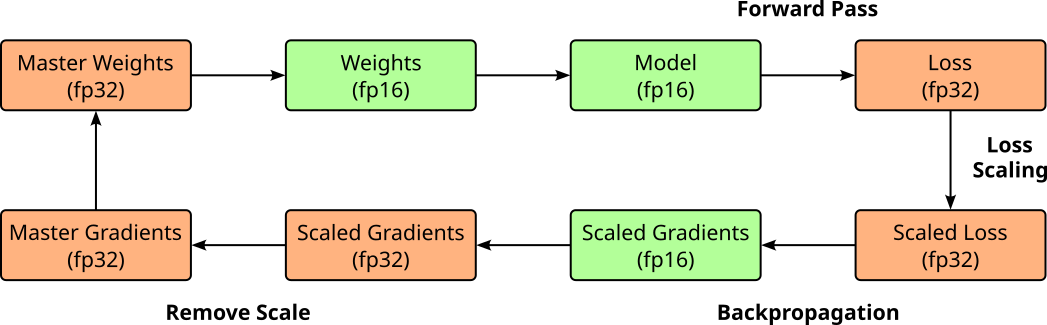
Mixed precision training has been shown to significantly improve training performance for large models, including large language models (LLMs), by reducing memory usage and increasing computational throughput. By performing most operations in FP16 while maintaining critical values like weight updates in FP32, it enables faster training on modern hardware — particularly GPUs with specialized support for half-precision arithmetic. Despite the reduced precision, mixed precision training achieves comparable accuracy to full FP32 training in practice. Techniques like loss scaling help preserve numerical stability, ensuring that model quality is not compromised. As a result, mixed precision has become a standard approach for efficiently training state-of-the-art neural networks at scale.
Summary
Quantization provides a practical way to reduce the memory footprint and computational requirements of neural networks by representing weights and activations with fewer bits. This is especially important for deploying large language models, where storing and processing billions of high-precision values can become prohibitively expensive. The notebook introduced the numerical foundations of fixed-point and floating-point representations and explained how these formats influence range and precision.
Although the basic idea of quantization is relatively straightforward, applying it successfully in practice presents a wide range of challenges. The choice between symmetric and asymmetric quantization affects both numerical accuracy and computational efficiency. Extreme values and outliers can dominate the quantization range, while clipping and rounding can remove or distort important information. Calibration is therefore essential for estimating suitable ranges and minimizing the resulting quantization error.
The notebook also examined the main approaches used in practice: Post-Training Quantization and Quantization-Aware Training. PTQ is relatively simple to apply but may degrade model quality when calibration data is not representative. QAT generally preserves accuracy more effectively by allowing the model to adapt to simulated quantization effects, but it makes training more complex. Through hands-on PyTorch examples, the notebook demonstrated why quantization is more than simply converting FP32 values to integers.
A solid understanding of these concepts is essential for deploying LLMs efficiently and reliably. Effective quantization requires balancing memory savings, inference performance, numerical precision, hardware support, and model accuracy; particularly when models must operate at large scale or on resource-constrained devices.