Disclaimer: This Jupyter Notebook contains content generated with the assistance of AI. While every effort has been made to review and validate the outputs, users should independently verify critical information before relying on it. The SELENE notebook repository is constantly evolving. We recommend downloading or pulling the latest version of this notebook from Github.
Dropout
As neural networks grow larger and more expressive, they become increasingly prone to overfitting: memorizing patterns in the training data rather than learning representations that generalize well to unseen examples. This risk is especially high in deep and overparameterized models, where many different parameter configurations can fit the training data equally well. Dropout was introduced as a simple yet powerful technique to combat this problem by injecting controlled randomness into the training process.
The core idea of dropout is to randomly deactivate neurons during training, forcing the network to rely on multiple alternative pathways to make predictions. Instead of allowing groups of neurons to co-adapt and specialize too narrowly, dropout encourages the learning of redundant, distributed representations. Each training step effectively uses a different subnetwork, making the overall model more robust to noise and small changes in the input.
From another perspective, dropout can be seen as an efficient way to approximate ensemble learning. Rather than explicitly training and storing many separate models, dropout trains a vast collection of subnetworks that all share parameters. At inference time, the full network acts like an average over these subnetworks, often leading to improved generalization and more stable predictions without additional computational cost.
Understanding dropout is important because it reveals how regularization, noise, and model capacity interact in deep learning. Dropout is not just a practical trick but a conceptual tool that illustrates why large neural networks can generalize despite often having far more parameters than training examples. Learning how and when to use dropout helps you design models that are both powerful and reliable, especially at scale.
Setting up the Notebook
Make Required Imports
This notebook requires the import of different Python packages but also additional Python modules that are part of the repository. If a package is missing, use your preferred package manager (e.g., conda or pip) to install it. If the code cell below runs with any errors, all required packages and modules have successfully been imported.
import numpy as np
Preliminaries
- This notebook assumes a basic understanding of calculus and the chain rules, including the general concept of backpropagation for training neural networks.
- While this notebook includes an implementation of dropout, this implementation is only for educational purposes. The institution is not to mimic highly optimized implementations provided by frameworks such as PyTorch or Tensorflow.
The Purpose of Dropout
Motivation
Modern neural networks are often overparameterized. This means that the network has more learnable parameters than are strictly necessary to fit the training data; often even more parameters than training examples. In this regime, there are many different parameter settings that achieve near-zero training error, so the model has a lot of freedom in how it represents the solution. This makes it easy for the network to fit complex patterns or even noise, but it also increases the risk of fragile solutions like co-adapted features unless something pushes the model toward simpler, more robust representations. Most modern networks are overparameterized by design because this regime actually makes optimization and representation learning easier. Wide and deep models have smoother loss landscapes, more redundant pathways, and are far less likely to get stuck in bad local minima, so gradient-based training works reliably. Overparameterization also lets the network discover rich, hierarchical features without us having to precisely engineer the architecture.
While overparameterization improves the model's capacity to learn, it also encourages redundancy which may cause a model to generalize poorly due to overfitting. A network with too much capacity often faces the following issues during training:
"Dead" neurons: When a network has far more neurons than it needs, not every neuron is required to contribute to minimizing the loss. During training, gradient descent may route useful computation through a subset of neurons while others: learn weights close to zero, activate extremely rarely, or learn features that get canceled out by later layers. These neurons do not hurt training loss, which also means that there is no strong pressure to make them useful.
Over-specialized neurons and co-adaption: The flip side of dead neurons are over-specialized neurons, i.e., the (potentially small) subset of neurons in the network have the most impact on the model's output. Over-specialization is the primary symptom of co-adaptation in overparameterized networks. Co-adaptation happens when neurons learn to be useful only in the presence of specific other neurons, instead of learning features that are independently meaningful. It is a situation where the network becomes lazy because neurons stop working independently and start relying on the specific outputs of their neighbors to get the right answer.
In general, we favour networks where most neurons contribute meaningfully to the output because it indicates that the network is using its capacity efficiently and robustly. When information is distributed across many neurons rather than concentrated in a small subset, the representation becomes less brittle: small changes, noise, or the failure of a single neuron are less likely to break the computation. This kind of distributed contribution is strongly associated with better generalization, since features that matter across many training examples tend to be reused and combined in stable ways instead of relying on narrow, accidental correlations.Note that "equal contribution" does not mean identical behavior but it means specialized neurons are individually useful, not dependent on a fragile web of other neurons to matter.
Basic Idea
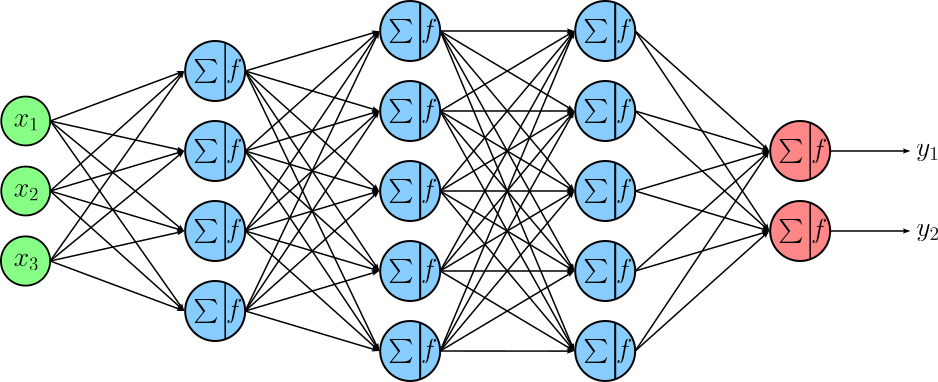
Dropout reduces the risks caused by overparameterization by randomly "turning off" (setting to zero) a subset of neurons during each training step. The hyperparameter of dropout is the probability $p$ of a neuron to be turned off. By doing this, the network is prevented from relying too heavily on any single neuron or small group of neurons. Each mini-batch effectively trains a slightly different sub-network, which forces the model to learn more robust and distributed representations rather than brittle, co-adapted features. To illustrate this, let's first consider a simple feedforward neural network (FNN) with $3$ hidden layers.
Dropout is typically applied after layers that produce activations, most commonly after fully connected (dense). The idea is to regularize feature representations, so dropout is placed after the linear transformation and nonlinearity, where neurons represent learned features that could otherwise co-adapt too strongly. Dropout is usually not applied to
- input layers (in a heavy way),
- the output layer,
- or during inference!
Applying dropout directly to the output layer can destabilize predictions, especially for classification or regression targets. It is also generally avoided in layers where information flow must be preserved precisely, such as batch normalization layers (dropout is placed after BN, not before) or recurrent connections in vanilla form, where naive dropout can break temporal consistency. If we apply dropout with a probability of $p=0.5$ to after all $3$ hidden layers of our example FNN, we might get the following setup where about half of the neurons in each layer are turned off (grey neurons).
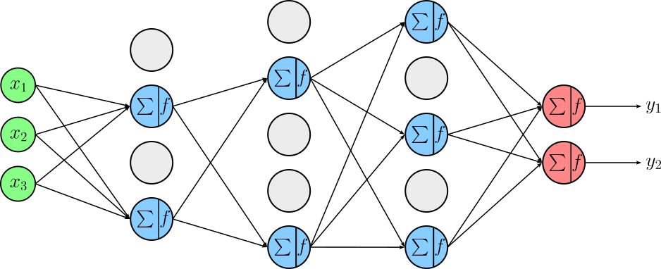
In practice, neurons that are turned off will receive an input as dropout is applied to the output. However, since their output is ignored through dropout, their inputs do not affect the computations. Thus, we can omit drawing the arrows that would otherwise point to these neurons.
As you can see from the figure above, using dropout can be understood as implicitly training an ensemble of many different subnetworks. Each time dropout is applied during training, a random subset of neurons is removed, which means the model being trained in that step is a slightly different architecture. Over the course of training, the shared weights are optimized across a huge number of these randomly sampled subnetworks, all of which overlap but differ in which units are active.
A key point about dropout** is that it is a training-time regularization technique only. During inference (testing or deployment), dropout is completely turned off and all neurons are active, which closely approximates averaging the predictions of this large ensemble. Instead of dropping units, the network uses appropriately scaled weights or activations so that the expected output matches what the model saw during training. This ensures deterministic, stable predictions: inference corresponds to using the full model, not a randomly thinned one.
Forward Pass
During the forward pass when training, input data is propagated layer by layer through the network, where each layer applies a linear transformation followed by a nonlinear activation function to produce intermediate activations. Training-specific components such as dropout or batch normalization (in training mode) may modify these activations. The final layer produces predictions, which are then compared to the ground-truth targets using a loss function to quantify how well the network is performing.
Considering dropout as one of the layers of a network architecture, it receives its input typically from the previous layer that produces activations. In the following, let's consider $\mathbf{X}$ the batched output of the 2nd or 3rd hidden layer of our example FNN; both have $5$ neurons. If we assume that the batch is of size $4$, $\mathbf{X}$ is a $4\times 5$ matrix:
Dropout effectively turns off neurons by setting their output to $0$ with probability $p$. In practice, this is typically implemented by defining a binary mask $\mathbf{M}$ with the same shape as $\mathbf{X}$ which is then multiplied with $\mathbf{X}$. A $0$ in mask $\mathbf{M}$ means that the output of a neuron is set to $0$; a $1$ in mask $\mathbf{M}$ means the output is "just passed through". In standard dropout, the dropout mask is sampled independently for each training sample, even when inputs are processed in a batch. That means different examples in the same batch will generally have different neurons turned off, which injects more noise and makes the regularization effect stronger and less correlated across samples. Thus, with $p=0.5$, the mask for our FNN may look as follows:
However, if this would be the final mask, we would have a problem: After applying dropout during training, the expected activation of the previous layer is reduced because a fraction of neurons are randomly set to zero. If nothing else were done, the average magnitude of activations flowing to the next layer would be smaller during training than during inference, when all neurons are active. This mismatch would cause the network to behave differently at test time, leading to systematically larger outputs and unstable predictions.
To fix this, the remaining active neurons are scaled up (typically by dividing by the keep probability $1-p$) during training, which is is known as inverted dropout. With this scaling, the expected value of each activation stays the same whether dropout is on or off. As a result, the network sees consistent activation statistics during training and inference, allowing dropout to act purely as a regularizer without changing the overall scale of the learned representations. To implement inverted dropout, we simply need to change the values of $1$ (reflecting the active neutrons) to $1/(1-p)$:
Thus, if $\mathbf{Y}$ denotes the output of the dropout layer, $\mathbf{Y}$ is computed as the Hadamard product (i.e., element-wise product) between input $\mathbf{X}$ and mask $\mathbf{M}$:
Output $\mathbf{Y}$ is now passed as input to any subsequent layer as part of the forward pass until it reaches the output layer yielding the final output of the network. During training, the final output is then used to compute the loss $\mathcal{L}$ based on the ground-truth labels from the training data. Of course, the goal is now to minimize the loss by performing backpropagation to compute the gradients with respect to all learnable parameters and the update those parameters accordingly.
Backward Pass
During the backward pass, the network computes gradients of the loss with respect to all trainable parameters by propagating error signals backward from the output layer to the input layers using the chain rule. Each layer uses the gradient of its output to calculate gradients for its weights, biases, and inputs, while training-specific operations like dropout block gradient flow through dropped neurons. These gradients are then used by an optimizer to update the parameters so that the loss is reduced in future forward passes.
Recall that our dropout received its input $\mathbf{X}$ as the output from a previous layer and passed its output $\mathbf{Y}$ to a subsequent layer. This means that during the backward pass, the dropout layer receives the computed upstream gradient $\frac{\partial \mathcal{L}}{\partial \mathbf{Y}}$ from the subsequent layer. Since loss $\mathcal{L}$ is a scalar and $\mathbf{Y}$ is matrix of shape $N\times M$, the gradient $\frac{\partial \mathcal{L}}{\partial \mathbf{Y}}$ will also have a shape of $N\times M$, with each element of $\frac{\partial \mathcal{L}}{\partial \mathbf{Y}}$ being the derivative of $\mathcal{L}$ with respect to one element in $\mathbf{Y}$. In other words, $\frac{\partial \mathcal{L}}{\partial \mathbf{Y}}$ is the Jacobian matrix (or just Jacobian), i.e., the matrix of all first-order partial derivatives of a function with multiple inputs and multiple outputs. It measures the sensitivity of each output component with respect to each input component. For our running example, the upstream gradient the dropout layer receives during the backward pass looks as follows:
The dropout layer itself has no learnable parameters (e.g., weights or biases). We therefore only need to compute the downstream gradient $\frac{\partial \mathcal{L}}{\partial \mathbf{X}}$ which is passed to the previous layer (with respect to the forward pass). By using the chain rule, we can compute the downstream gradients as:
Even without computing the downstream gradient, we already know the shape the Jacobian $\frac{\partial \mathcal{L}}{\partial \mathbf{X}}$ must have. Again, since loss $\mathcal{L}$ is a scalar value, the shape of the Jacobian must be the as the one of $\mathbf{X}$ — more our example: $\frac{\partial \mathcal{L}}{\partial \mathbf{X}} \in \mathbb{R}^{4\times 5}$. We can now look at the individual values $\frac{\partial \mathbf{Y}}{x_{ij}}$. For this, we need to distinguish two cases:
Neuron was turned off: If the $j$-th neuron was turned off for the $i$-th data sample, $y_{ij} = 0$. In this case, the gradient $\frac{\partial \mathbf{Y}}{x_{ij}}$ is just $0$.
Neuron was active: If the $j$-th neuron was turned off for the $i$-th data sample, $y_{ij} = x_{ij}/(1-p)$. In this case, the gradient $\frac{\partial \mathbf{Y}}{x_{ij}}$ is $1/(1-p)$.
Important: In principle, to compute $\frac{\partial\mathcal{L}}{\partial x_{ij}}$, we must account for every path through which $x_{ij}$ influences (or might influence) the loss $\mathcal{L}$. However, we know — and the forward pass makes it obvious, we know that the value of $y_{ij}$ only depends on $x_{ij}$ (and whether the neuron was active or turned off). In other words, there is only one path from $x_{ij}$ to $\mathcal{L}$ and it goes through $y_{ij}$.
If you look closely at all partial derivatives $\frac{\partial \mathbf{Y}}{x_{ij}}$, you will notice that the downstream gradient $\frac{\partial \mathcal{L}}{\partial \mathbf{X}}$ is the same as mask $\mathbf{M}$. In short, for the dropout layer in our example FNN, we get:
This convenient result highlights the simplicity of the idea of dropout and makes it very easy to implement dropout as a network layer, which we will look into next.
Basic Implementation
Deep learning frameworks like PyTorch and TensorFlow typically structure neural networks as collections of layer objects, where each layer is implemented as its own class with a forward() method that defines how inputs are transformed into outputs. Conceptually, each layer also has a corresponding backward() method, which computes gradients with respect to its inputs and parameters during the backward pass. This design makes models modular and composable, so layers can be easily reused, stacked, swapped, or extended. It also improves clarity and debuggability, since each layer encapsulates its own behavior and parameters. Finally, it enables powerful optimizations: frameworks can automatically build computation graphs, efficiently compute gradients, and run parts of the model on different hardware (CPU/GPU) without the user needing to manage low-level details.
The class Dropout follows this design to implement a dropout layer using only NumPy. Notice that the class also implements two methods train() and eval() — this naming is in line with the PyTorch library to set the class variable self.train to True or False. This class variable tells the dropout layer of the model is in training mode or and inference mode. Since no neurons are turned off in inference mode, the forward() method will just pass through the input $\mathbf{X}$, and the backward() method will pass through the upstream gradient $\frac{\partial \mathcal{L}}{\partial \mathbf{Y}}$. The same is true when $p=0.0$, i.e., no neuron is turned off during training.
class Dropout:
    def __init__(self, p=0.5):
        assert 0 <= p < 1     # Make sure that p is a valid probability value
        self.p = p
        self.mask = None
        self.train = True

    def forward(self, X):
        # Do nothing if an evaluation/inference mode or p=0.0
        if not self.train or self.p == 0:
            return X

        # Inverted dropout mask
        self.mask = (np.random.rand(*X.shape) > self.p) / (1 - self.p)
        return X * self.mask

    def backward(self, dY):
        # Return downstream gradeint "as is" if an evaluation/inference mode or p=0.0
        if not self.train or self.p == 0:
            return grad_output
        #Compute downstream gradient via chain rule (upstream gradient * mask)
        return dY * self.mask

    def train():
        self.train = True

    def eval():
        self.train = False
To test the implementation, we first have to define some random input $\mathbf{X}$. In line with our running example we define $\mathbf{X}$ as an input matrix of shape $4\times 5$.
X = np.array(np.arange(20)).reshape(4, 5) / 20

print(f"Input X:\n{X}")
Input X:
[[0.   0.05 0.1  0.15 0.2 ]
 [0.25 0.3  0.35 0.4  0.45]
 [0.5  0.55 0.6  0.65 0.7 ]
 [0.75 0.8  0.85 0.9  0.95]]
For the backward pass, we also need some upstream gradient $\frac{\partial \mathcal{L}}{\partial \mathbf{Y}}$ of the same shape.
dY = np.array(np.arange(20)).reshape(4, 5) / 50

print(f"Upstream Gradient dY:\n{dY}")
Upstream Gradient dY:
[[0.   0.02 0.04 0.06 0.08]
 [0.1  0.12 0.14 0.16 0.18]
 [0.2  0.22 0.24 0.26 0.28]
 [0.3  0.32 0.34 0.36 0.38]]
Let's create an instance of the Dropout class with a probability of $p=0.5$. This means, of course that the keep probability $(1-p)$ will also be $0.5$.
dropout = Dropout(p=0.5)
To compute the output Y of the dropout layer as part of the forward pass, we pass X to the forward(). Note that we also set a random seed in the code cell below. This is only here to ensure that the mask will always be the same for consistency; in practice, we obviously would not do this. The forward() method also stores the mask as a class variable self.class since we need to use the same mask again for the backward pass.
np.random.seed(1)

Y = dropout.forward(X)
For this example, we do not really care about the output Y which would be passed to the next layer as input in a complete model architecture. However, let's have a look at the mask that was generated as part of the forward() method.
print(f"Dropout mask:\n{dropout.mask}")
Dropout mask:
[[0. 2. 0. 0. 0.]
 [0. 0. 0. 0. 2.]
 [0. 2. 0. 2. 0.]
 [2. 0. 2. 0. 0.]]
The $0$s in the mask reflect the neurons that have been turned off; the $2$ reflect the scaling factor $1/(1-p)$ with $p=0.5$. Output Y is, of course, the Hadamard Product between X and self.mask; see the expression X * self.mask.
Performing the backward pass is equally straightforward as we already know that the downstream gradient $\frac{\partial \mathcal{L}}{\partial \mathbf{X}}$ is simply the result of the Hadamard Product between the upstream gradient the dropout layer receives during backpropagation and the mask, which we computed during the forward pass. Again, we only need to perform this product in training mode and when $p > 0.0$.
dX = dropout.backward(dY)

print(dX)
[[0.   0.04 0.   0.   0.  ]
 [0.   0.   0.   0.   0.36]
 [0.   0.44 0.   0.52 0.  ]
 [0.6  0.   0.68 0.   0.  ]]
dX now holds the downstream gradient $\frac{\partial \mathcal{L}}{\partial \mathbf{X}}$ which is finally passed to the previous layer (with respect to the forward pass) to continue the backward pass to the input layer. As the dropout layer itself has no learnable parameters, there are also no parameters to be changed in the update step of backpropagation.
Discussion
In the previous section, we introduced the most basic version and implementation of dropout, i.e., the random turning off of neurons given a probability $p$. While this implementation of dropout is arguably still the most commonly used variant, improvements of the original idea have been proposed. In the following, we briefly outline some of those improvements or otherwise alternative variants of Dropout.
Sampling Strategies
So far, we only mentioned that the masking of a neuron depends on a probability $p$. However, we did not go into details about how $p$ to make this decision. Most commonly, For each neuron (or activation), a random variable is sampled from a Bernoulli distribution to decide whether that neuron is kept or turned off. A Bernoulli distribution naturally models a coin flip because it represents the simplest possible random experiment with two outcomes: success or failure, on or off, keep or drop. When the probability is $p = 0.5$, the coin is fair and both outcomes are equally likely, but the same abstraction applies when $p \neq 0.5$: the coin is simply biased. This simple strategy allows for the straightforward scaling of the remaining active neurons by factor$1 / (1 - p)$ to ensure that the expected value of each activation remains unchanged between training and inference
Beyond standard Bernoulli masking, several alternative strategies exist. For example Gaussian dropout, the binary mask is replaced by multiplicative Gaussian noise with mean 1 and variance determined by $p$, approximating Bernoulli dropout in expectation. Structured dropout variants (e.g. spatial dropout or DropBlock) use the same probability $p$ but apply it to groups of neurons such as entire channels or contiguous regions rather than individual units. Finally, in adaptive or Bayesian variants like Concrete Dropout, $p$ itself can be learned from data, allowing the model to decide which parts should be dropped more aggressively. In short, while the core idea is always to use $p$ as the probability of suppressing information flow, practical implementations differ in how the mask is sampled, how scaling is handled, and at what structural level the decision is applied.
Dropout Variants
Although "dropout" is often spoken of as a single technique, in practice it refers to a family of related regularization methods built around the same core idea: deliberately injecting noise by randomly disabling parts of a model during training. Different architectures impose different structural constraints — spatial locality in CNNs, temporal consistency in RNNs, depth and residual pathways in Transformers. As a result, dropout has evolved into multiple variants that drop neurons, connections, feature maps, blocks, or even entire layers, and that may use fixed, adaptive, or learned dropout rates. Framing dropout as a family of methods highlights that its essence lies not in what is dropped, but in how stochastic regularization is matched to the model's structure and learning dynamics. The following list outlines some of the more popular variants beyond the basic dropout:
DropConnect: This variant extends the intuition of dropout by randomly removing connections (weights) rather than entire neuron activations during training. This injects noise at the parameter level, encouraging the network to avoid relying too heavily on specific connections and to distribute information more robustly across many weights. In practice, DropConnect is most commonly associated with fully connected layers in FNNs, where large dense weight matrices are prone to overfitting. It has also been explored in recurrent networks (notably early LSTM variants) to regularize large hidden-to-hidden weight matrices, though it is less common there today due to optimization difficulties.
Spatial Dropout (Channel Dropout): Spatial Dropout is motivated by the observation that in convolutional layers, neighboring activations within a feature map are highly correlated. Dropping individual activations therefore injects little effective noise and can even harm spatial coherence. Spatial Dropout addresses this by randomly dropping entire feature maps (channels) instead of individual pixels, forcing the network to avoid relying too heavily on any single convolutional filter and to learn more redundant, robust representations. It is therefore most commonly used in convolutional neural networks (CNNs), particularly in deeper layers where feature maps represent higher-level concepts.
Variational Dropout: Variational Dropout is most commonly used in recurrent neural networks**, including RNNs, LSTMs, and GRUs, where preserving temporal structure is essential. It is motivated by the instability that arises when standard dropout applies a different random mask at every time step in a sequence. In recurrent settings, this introduces rapidly changing noise that can disrupt temporal credit assignment and memory. Variational Dropout fixes this by sampling a single dropout mask per sequence and reusing it across all time steps, making the injected noise consistent over time while still providing regularization.
Recurrent Dropout: As another dropout variant to be used in RNNs/LSTMs/GRUs, Recurrent Dropout is designed to regularize the hidden-to-hidden connections in recurrent networks without disrupting the temporal dynamics of the sequence. Instead of applying dropout independently at each time step (which can destabilize learning), a fixed dropout mask is applied to the recurrent connections across all timesteps, preventing over-reliance on specific hidden units while maintaining consistent signal flow through time. By focusing on the recurrent pathways rather than input-to-hidden connections, it preserves the network's memory while still providing effective stochastic regularization.
Stochastic Depth (LayerDrop): Stochastic Depth (also called LayerDrop) extends the dropout idea from neurons to entire layers: during training, each residual or feedforward layer is randomly skipped with a certain probability. This forces the network to learn robust representations that do not rely on any single layer, effectively creating an ensemble of networks of varying depth and reducing overfitting. It also has the added benefit of reducing computation during training since some layers are bypassed. Stochastic Depth is most commonly used in very deep architectures with residual connections, such as ResNets and deep Transformers, where skipping layers does not break gradient flow due to the skip connections. It is particularly valuable in extremely deep models where overfitting or vanishing gradients could otherwise become a problem.
Practical Considerations
When applying dropout in practice, several considerations matter beyond simply inserting a dropout layer. In general, the place of the dropout layer is crucial. Dropout is typically applied after nonlinearities or between blocks, while early layers (especially in CNNs) often use little or no dropout because they learn low-level, broadly useful features. Interaction with other regularizers also matters. Strong data augmentation, weight decay, batch normalization, or very large datasets can reduce or even eliminate the need for dropout, and combining all of them aggressively can lead to underfitting. Finally, dropout increases gradient noise, which can slow convergence; learning rates, training time, or warm-up schedules may need adjustment.
As for the dropout probability $p$ (the probability of turning off a neuron), common practical choices are fairly conservative. For fully connected layers, values around $p = 0.5$ are classic and still widely used, while $p = 0.1$ to $p = 0.3$ is typical for convolutional layers or transformer sublayers. Embeddings and attention layers often use even smaller rates (e.g. $0.05$ to $0.1$), since excessive dropout there can harm representation learning. In very deep or overparameterized models, dropout rates are often reduced rather than increased, and sometimes replaced by structured methods like stochastic depth. In short, dropout probabilities are usually chosen small enough to regularize without disrupting the model's core signal, and are tuned in conjunction with model size, data volume, and other regularization techniques.
Summary
This notebook introduced dropout as a fundamental regularization technique for neural networks, motivated by the problem of co-adaptation and overfitting in large, overparameterized models. At its core, dropout injects stochasticity during training by randomly disabling units, forcing the network to learn more robust, distributed representations. Although the idea is conceptually simple, it has far-reaching effects on optimization, generalization, and model design.
We formalized dropout mathematically by deriving the forward pass, where activations are element-wise masked and rescaled using inverted dropout to preserve the expected activation magnitude. Building on this, we examined the backward pass, showing how gradients flow only through the active units and are scaled consistently with the forward computation. These derivations clarify that dropout is not merely a heuristic, but a well-defined stochastic transformation that integrates cleanly into gradient-based learning.
To make these ideas concrete, the notebook implemented dropout from scratch using NumPy only, exposing the mechanics that deep learning frameworks usually hide. Writing explicit forward() and backward() methods highlighted how the dropout mask must be stored during training, how gradients are masked during backpropagation, and how behavior differs between training and inference modes. This low-level implementation reinforces an intuitive understanding of what dropout actually does inside a network.
Finally, the notebook emphasized that, despite its simplicity, effective use of dropout in practice is subtle. Choices about where to apply dropout, how large the dropout probability should be, and how it interacts with other regularization techniques and architectural components can strongly influence training dynamics and final performance. Dropout is best understood not as a single plug-and-play trick, but as part of a broader design space of stochastic regularization methods that must be adapted carefully to the model and task at hand.