Disclaimer: This Jupyter Notebook contains content generated with the assistance of AI. While every effort has been made to review and validate the outputs, users should independently verify critical information before relying on it. The SELENE notebook repository is constantly evolving. We recommend downloading or pulling the latest version of this notebook from Github.
Layer Normalization
Training deep neural networks is often challenging because the distribution of activations inside the network can change throughout training. As parameters are updated, the inputs to intermediate layers may shift in scale and distribution, making optimization unstable and slowing convergence. These issues become especially pronounced in very deep architectures or sequence models, where small changes can accumulate across many layers and time steps. As a result, practitioners have developed normalization techniques that stabilize activations and improve the efficiency of gradient-based learning. Layer normalization is one such technique. It computes normalization statistics across the features of a single training example. By maintaining more consistent activation scales, layer normalization can improve optimization stability, accelerate training, and enable deeper and more expressive architectures.
Normalization methods have become a foundational component of modern deep learning systems. Techniques such as layer normalization, batch normalization, group normalization, and RMS normalization are now routinely integrated into state-of-the-art neural network architectures. In particular, layer normalization plays a central role in transformer-based models, including large language models and many recent advances in natural language processing, vision, and multimodal learning. Understanding how and why these normalization methods work is therefore essential for anyone studying contemporary machine learning.
In this notebook, we will explore the motivation, mathematical formulation, and implementation details of layer normalization. By the end, you should have both a conceptual and practical understanding of layer normalization and its role in deep learning.
Setting up the Notebook
Make Required Imports
This notebook requires the import of different Python packages but also additional Python modules that are part of the repository. If a package is missing, use your preferred package manager (e.g., conda or pip) to install it. If the code cell below runs with any errors, all required packages and modules have successfully been imported.
import numpy as np
Preliminaries
- This notebook assumes a basic understanding of calculus and the chain rules, including the general concept of backpropagation for training neural networks.
- While this notebook includes an implementation of a layer normalization, this implementation is only for educational purposes. The institution is not to mimic highly optimized implementations provided by frameworks such as PyTorch or Tensorflow.
Motivation
The Goal
Training a neural network is fundamentally an optimization problem: we want gradient-based methods such as stochastic gradient descent to steadily improve the model parameters. This process becomes much easier when the distribution of activations in each layer remains relatively stable throughout training. If the activations of a layer constantly shift in scale or mean as earlier layers change, then downstream layers must continuously adapt to new input distributions. This phenomenon is often referred to as internal covariate shift (although the exact interpretation is debated), and it can make optimization slower and less stable. Stable activation distributions provide several important benefits:
Preserve "healthy" ranges for gradients: If activations become extremely large or small, gradients can explode or vanish as they propagate through the network, especially in deep architectures. Keeping activations well-scaled allows gradients to flow more reliably across many layers, which improves learning dynamics and enables deeper models to train effectively.
Predictable input space: When the statistics of a layer’s inputs change dramatically from one training step to the next, the layer must repeatedly readjust its parameters to compensate. This can slow convergence because the optimization target is effectively moving during training. The goal is to reduce these shifts, allowing layers to focus on learning meaningful representations rather than constantly adapting to changing input scales.
More robust hyperparameter choices Networks with stable activations typically tolerate larger learning rates and converge faster because the optimization landscape becomes smoother and better conditioned.
The Problem
When training deep neural networks, normalization is not just about scaling the input features to a common range. Even if the input is perfectly normalized, the representations inside the network — the hidden activations $\mathbf{a}^{[l]}$ — are repeatedly transformed by learned weight matrices and nonlinearities. As training progresses, updates to earlier layers continuously change the distribution of these intermediate features. To better illustrates, consider the $l$-th hidden layer in a basic artificial neural network; assuming a simple linear layer, its activation $\mathbf{a}^{[l]}$ is computed as:
where $\mathbf{W}^{[l]}$ and $\mathbf{b}^{[l]}$ are the weight matrix and the bias terms, and $f^{[l]}$ is some nonlinear activation function (e.g., ReLU, Sigmoid, Tanh); $\mathbf{a}^{[l-1]}$ is the activation (i.e., the output) of the previous layer at $(l\!-\!1)$. We also assume a $(l\!+\!1)$-th hidden layer which receives $\mathbf{a}^{[l]}$ as its input.
When training the network, weight matrix $\mathbf{W}^{[l]}$ and bias vector $\mathbf{b}^{[l]}$ get updated after backpropagation to compute all gradients. Depending on the changes in $\mathbf{W}^{[l]}$ and $\mathbf{b}^{[l]}$ the distribution of activations $\mathbf{a}^{[l]}$ may noticeable change. Moreover, since this is true for all layers, the distribution of activations $\mathbf{a}^{[l-1]}$ of the preceding layer, which further adds to the effect on $\mathbf{a}^{[l]}$. While these effects might be small, they can compound across layers in deep networks, i.e., networks with many layers as each layer's output depends on all previous layers. To visualize this, the plot below shows the distribution of activations of a deep hidden layer after several epochs of training.
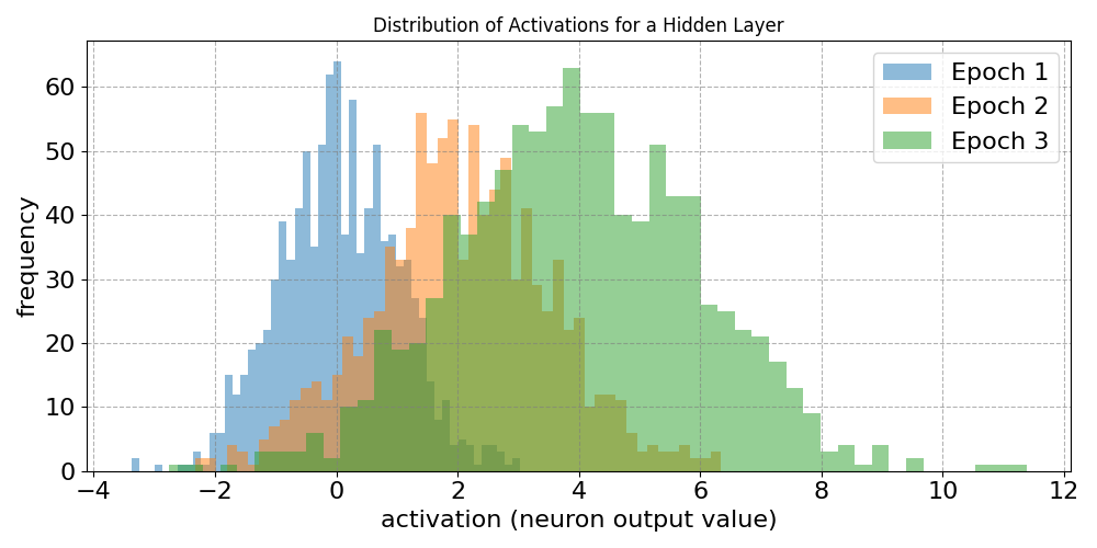
Notice that both the mean and variance of the distribution drifts over time (i.e., across epochs). This effect is independent from whether the training data was normalized or not. In other words, particularly in the context of deep neural networks, normalization issues reappear inside the network, even if the external input was well behaved.
Layer Normalization — Overview
Internal normalization refers to normalization techniques that are applied inside a model during training, rather than preprocessing the input data beforehand. The term is most commonly used in the context of neural networks because deep networks consist of many stacked layers whose activation distributions continuously change during training ($\rightarrow$ internal covariate shift; see above). Instead of normalizing features once before feeding them into the model (external normalization), internal normalization adjusts the distributions of intermediate activations within the network itself. The goal is to keep layer inputs in a stable and well-behaved range (e.g., controlled mean and variance), which improves optimization, stabilizes gradients, and accelerates convergence.
Because of their importance, a wider range of normalization strategies have been proposed, including Layer Normalization, Batch Normalization, Instance Normalization, Group Normalization, Weight Normalization, Spectral Normalization, RMS Normalization. The choice of normalization method strongly depends on architecture and batch size: CNNs often use Batch, Group, or Instance Normalization; recurrent networks and transformers typically rely on Layer Normalization or RMS Normalization; and generative models like GANs may additionally use Spectral Normalization for stability.
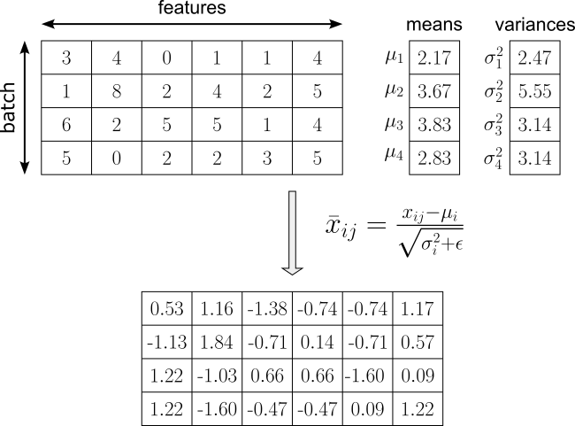
The focus of this notebook is on Layer Normalization which works by normalizing the activations of a single data sample across its feature dimensions, rather than across the batch. For each individual example, it computes the mean and variance over all features in a given layer, then subtracts the mean and divides by the standard deviation (with a small constant added for numerical stability); see this step for our example output in the figure below.
Since each sample has again zero mean and unit variance, Layer Normalization also introduces learnable scaling and shifting parameters. In fact, the learnable scaling parameters are still defined per feature dimension (not per sample). Thus, there is again one $\gamma_j$ and one $\beta_j$ for each feature $j$, shared across all samples, resulting the the same formula:
The key advantage of Layer Normalization is that it does not depend on mini-batch statistics. Because normalization is performed independently for each sample across its feature dimensions, it works reliably with small batch sizes and even batch size 1. It also behaves identically during training and inference, avoiding discrepancies between batch statistics and running averages. This makes it particularly well-suited for sequence models such as recurrent neural networks and transformer architectures, where batch sizes may vary or temporal dependencies make batch-wise normalization less appropriate. On the flip side, Layer Normalization does not benefit from the regularizing effect that arises from noisy batch statistics in Batch Normalization. It may also be less effective in convolutional neural networks, where feature-wise normalization across spatial dimensions can sometimes better exploit the structure of image data. In practice, while it improves training stability, it often does not accelerate convergence in feedforward or convolutional networks as strongly as batch normalization does.
Let's define the input batch from the example above as a NumPy array for later when implementing Layer Normalization from scratch. Throughout the notebook, we use $N$ and $D$ to denote the number of samples in the batch and the number of features of each sample, respectively.
batch = np.asarray([
    [3, 4, 0, 1, 1, 4],
    [1, 8, 2, 4, 3, 5],
    [6, 2, 5, 5, 1, 4],
    [5, 0, 2, 2, 3, 5]
])

N, D = batch.shape

print(f"Number of samples: {N}")
print(f"Number of features: {D}")
Number of samples: 4
Number of features: 6
Forward Pass
The forward pass in a neural network is the process where input data moves layer by layer through the network to produce an output or prediction. At each layer, the network applies mathematical operations such as matrix multiplication, adding biases, and activation functions to transform the data into increasingly useful representations. For Layer Normalization, the forward pass consists of two main steps: the basic normalization, and then the scaling & shifting. In the normalization step, the activations within a layer are standardized by subtracting their mean and dividing by their standard deviation, which helps stabilize training and improve convergence. After normalization, the model applies learnable scaling and shifting parameters so the network can adjust the normalized values if needed. This combination maintains stable activations while preserving the flexibility of the model.
Basic Normalization
When we normalize values by subtracting the mean and dividing by the standard deviation, each resulting value represents how many standard deviations it is away from the mean. A positive normalized value means the original value was above the mean, while a negative value means it was below the mean. For example, a normalized value of $2$ indicates the original value was two standard deviations above the average. This process transforms the data into a standardized scale with mean $0$ and variance $1$, making different features or activations easier to compare and process consistently.
In the context of Layer Normalization, this standardization helps stabilize the activations flowing through the neural network. Since the values are kept within a more controlled range, the network becomes less sensitive to extreme activation values and changes in scale between layers. This improves training stability, allows gradients to flow more smoothly during backpropagation, and often leads to faster convergence. By ensuring that activations are expressed relative to their distribution rather than their raw magnitude, Layer Normalization helps the model learn more efficiently and consistently across different inputs.
Computing the mean $\mu_i$ for the $i$-th sample in a batch is defined as:
To compute the standard deviation $\sigma_i$ for the $i$-th sample, we first compute its variance $\sigma_i^2$ which is defined as
In short, variance tells us the average amount by which values deviate from the mean. Before computing the standard deviation $\sigma_i$, which is just the square root of the variance $\sigma_i^2$, we first add a small value $\epsilon$ (common: $\epsilon = 10^{-5}$) to the variance. The reason for this is to later avoid any division by $0$ — this could happen if all $x_{ij}$ values of the $i$-th sample are the same; which also means that the mean would be the same value.
With this, we can compute the normalized value $\hat{x}_{ij}$ for each $x_{ij}$ of the $i$-th sample as:
Side note: Why $\sqrt{\sigma_i^2 + \epsilon}$ instead of $\sqrt{\sigma_i^2} + \epsilon$? While both alternatives ensure that we do not divide by $0$ during the forward pass, only the former expression ensures that we also do not divide by $0$ during the backward pass. To see this let's first consider the function $f(v) = \sqrt{v + \epsilon}$. During backpropagation we need to compute the derivative $df/dv$ which is:
Thus, even if $v=0$, we always avoid dividing by $0$. Now let's assume the function $f(v) = \sqrt{v} + \epsilon$ with the following derivative:
Now if $v=0$, we would divide by $0$. This is the reason why add $\epsilon$ to the variance $\sigma_i^2$ and compute the square root to get the deviation value we use for the normalization step.
To make our lives a bit easier throughout the notebook, let's define $\large\sigma_{i,\epsilon} = \sqrt{\sigma_i^2 + \epsilon}$ to get:
This little custom notation is merely to simplify the representation, which will come very handy when to come the backward pass and the many partial derivatives we need to compute for all involved chain rules. Lastly, if we denote $\mu$ to be the vector of means and $\sigma_\epsilon$ to be the vector of standard deviations for all samples in input batch $\mathbf{X}$, we can write the normalization step in a vectorized form:
Note that subtracting a vector from a matrix or dividing a matrix by a vector assumes broadcasting, which allows arrays with different shapes to work together in arithmetic operations by virtually expanding the smaller array to match the dimensions of the larger one.
Using the definitions above we can directly implement the normalization step using NumPy in Python. The normalize() method performs feature normalization on each row of the input matrix X. To this end, it first computes the mean and variance across the features in each row with np.mean() and np.var() using axis=1, while keepdims=True preserves the matrix dimensions for broadcasting. The function then subtracts the mean from each value and divides by the square root of the variance plus a small constant eps representing $\epsilon$.
def normalize(X, eps=1e-5):
    # Compute mean and variance across features
    mean = np.mean(X, axis=1, keepdims=True)
    var = np.var(X, axis=1, keepdims=True)
    # Normalize and return batch
    return (X - mean) / np.sqrt(var + eps)
Let's apply the method normalize() to our example batch we define above. Of course, the result should match the one shown in the previous figure.
batch_normalized = normalize(batch)

with np.printoptions(precision=2, suppress=True):
    print(batch_normalized)
[[ 0.53  1.17 -1.38 -0.74 -0.74  1.17]
 [-1.25  1.84 -0.81  0.07 -0.37  0.51]
 [ 1.22 -1.03  0.66  0.66 -1.6   0.09]
 [ 1.22 -1.6  -0.47 -0.47  0.09  1.22]]
Scaling & Shifting
As mentioned before, after the basic normalization step, the output for each sample will have, by definition, a mean of $0$ and a variance of $1$. While this is great for stabilizing early training and preventing exploding/vanishing gradients, it may also remove information about the original scale and distribution of the outputs. Layer Normalization therefore introduces two learnable parameters $\gamma$ (initialized to $1$) and $\beta$ (initialized to $0$) allow the network to "undo" the normalization if that is what the model determines is best for minimizing the loss.
The parameters $\gamma$ and $\beta$ are defined per feature rather than per sample because features represent consistent dimensions of the data across all samples. Each feature may require a different adjustment after normalization, so assigning separate learnable parameters to each feature allows the network to learn how important or influential that feature should be. For example, the model might learn: "Feature $j$ is highly sensitive and needs a wide dynamic range ($\gamma_j$), while feature $k$ needs to be tightly bounded." If scaling and shifting were defined per sample instead, the parameters would depend on individual inputs rather than the structure of the features themselves.
As such $\gamma$ and $\beta$ are vectors of size $D$. With $\gamma_j\in\gamma$ and $\beta_j\in\beta$, we can define the final output of Layer Normalization for a single value as:
We can also write this computation in vectorized form to apply the scaling and shifting to the normalized batch $\hat{\mathbf{X}}$:
Important: Saying $\gamma$ and $\beta$ can "undo" the normalization does not mean the layer reverts to the wild, unpredictable, and shifting distributions we had before normalization was applied. Because the same $\gamma$ and $\beta$ values are applied to all $\hat{x}_{ij}$ values at a layer during an epoch, the outputs remain bound to a tightly controlled distribution. The distribution is allowed to stretch and shift into an optimal shape, but it is anchored by these parameters. In simple terms, the distributions still remain stable across epochs, but are no longer forced to have a mean of $0$ and a variance of $1$.
To show scaling and shifting in action let's define a $\gamma$ and a $\beta$ vector using NumPy arrays; see the code cell below. Notice that we initialize $\gamma$ with all $1$s and $\beta$ with all $0$s. Of course, the size of both vectors reflects the number of features $D$.
gamma = np.ones((1, D))
beta = np.zeros((1, D))
Since NumPy automatically uses broadcasting for matching shapes, implementing the scaling and shifting steps is straightforward.
batch_final = gamma * batch_normalized + beta

with np.printoptions(precision=2, suppress=True):
    print(batch_final)
[[ 0.53  1.17 -1.38 -0.74 -0.74  1.17]
 [-1.25  1.84 -0.81  0.07 -0.37  0.51]
 [ 1.22 -1.03  0.66  0.66 -1.6   0.09]
 [ 1.22 -1.6  -0.47 -0.47  0.09  1.22]]
Since all $\gamma_j = 1$ and all $\beta_j = 0$, the result naturally matches the output of the normalization step since we actually did not scale or shift any value. Of course, during training, all $\gamma_j$ and $\beta_j$ values are likely to change and this resulting and truly scaled and shifted values.
To sum up, the forward pass of Layer Normalization is relatively straightforward because it mainly consists of computing the mean and variance, normalizing the activations, and then applying learnable scaling and shifting parameters. These operations are conceptually simple and can be implemented concisely using matrix operations and broadcasting. As a result, the forward computation is both intuitive and computationally efficient. The backward pass, however, is considerably more involved. In particular, the derivatives of the basic normalization step introduce non-trivial dependencies between inputs, making the backward pass mathematically more complex than the forward pass.
So this is what we need to check out next.
Backward Pass
The backward pass in a neural network is the process of propagating gradients from the output layer back through the network in order to update the model's parameters. Using the chain rule from calculus, the network computes how much each parameter contributed to the final error or loss. These gradients are then used by optimization algorithms such as gradient descent to adjust the weights and biases so the model can improve its predictions over time.
For Layer Normalization, the backward pass means computing gradients not only through the learnable scaling and shifting parameters, but also through the normalization operation itself. This is more complicated because each normalized value depends on the mean and variance of all features within the same sample. As a result, the gradient for one feature is influenced by the other features in the layer. The backward pass therefore requires carefully differentiating through the computations for the mean, variance, standard deviation, and normalization steps so that accurate gradients can be propagated back to earlier layers in the network.
In the following, we assume that Layer Normalization is some layer in the network — that is; it received its input $\mathbf{X}$ as the output from a previous layer and passed its output $\mathbf{Y}$ to a subsequent layer. The latter assumes that during the backward pass through the Layer Normalization layer, the upstream gradient $\frac{\partial \mathcal{L}}{\partial \mathbf{Y}}$ has been computed. Since loss $\mathcal{L}$ is a scaler and $\mathbf{Y}$ is matrix of shape $N\times M$, the gradient $\frac{\partial \mathcal{L}}{\partial \mathbf{Y}}$ will also have a shape of $N\times M$, with each element of $\frac{\partial \mathcal{L}}{\partial \mathbf{Y}}$ being the derivative of $\mathcal{L}$ with respect to one element in $\mathbf{Y}$. In other words, $\frac{\partial \mathcal{L}}{\partial \mathbf{Y}}$ is the Jacobian matrix (or just Jacobian), i.e., the matrix of all first-order partial derivatives of a function with multiple inputs and multiple outputs. It measures the sensitivity of each output component with respect to each input component. For our example batch of shape $(4, 6)$, the upstream gradient we start with looks as follows:
During the backward pass through the Layer Normalization layer we nee to compute several gradients:
The downstream gradient $\frac{\partial \mathcal{L}}{\partial \mathbf{X}}$ to be passed to the next layer of the backward pass (i.e., the layer preceding the Layer Normalization layer in the overall architecture)
The gradients $\frac{\partial \mathcal{L}}{\partial \mathbf{\gamma}}$ and $\frac{\partial \mathcal{L}}{\partial \mathbf{\beta}}$ to update the learnable parameters $\gamma$ and $\beta$ for the scaling and shifting step
By using the chain rule of Calculus, we can calculate these gradients as follows:
$\large \frac{\partial\mathcal{L}}{\partial\mathbf{Y}}$ is of course the upstream gradient we receive from the previous layer with respect to the backward pass. This means we now have to compute the gradients, i.e., the Jacobians, $\large \frac{\partial\mathbf{Y}}{\partial\mathbf{X}}$, $\large\frac{\partial\mathbf{Y}}{\partial\mathbf{\gamma}}$, and $\large \frac{\partial\mathbf{Y}}{\partial\mathbf{\beta}}$. In fact, we need $\large\frac{\partial\mathbf{Y}}{\partial\mathbf{\gamma}}$ and $\large \frac{\partial\mathbf{Y}}{\partial\mathbf{\beta}}$ to compute $\large \frac{\partial\mathbf{Y}}{\partial\mathbf{X}}$ since Layer Normalization involves the two steps of basic normalization and shifting & scaling — but for the backward pass we have to go the other direction.
Backward Pass through Scaling & Shifting
With respect to scaling and shifting, its input is the batch $\hat{\mathbf{X}}$; recall:
This means that apart from $\large\frac{\partial \mathcal{L}}{\partial \mathbf{\gamma}}$ and $\large\frac{\partial \mathcal{L}}{\partial \mathbf{\beta}}$, we also need to compute the "intermediate" downstream gradient $\large\frac{\partial \mathcal{L}}{\partial \hat{\mathbf{X}}}$ we then pass to the backward pass through the basic normalization. So let's do this step by step.
Computing $\large\frac{\partial \mathcal{L}}{\partial \gamma}$
Recall that $\gamma$ is a $D$-dimensional vector with $D$ being the number of features. This implies that $\large\frac{\partial \mathcal{L}}{\partial \gamma}$ is a $D$-dimensional vector as well. We therefore start by computing $\large\frac{\partial \mathcal{L}}{\partial \gamma_j}$, i.e., the partial derivative with respect to $\gamma$ value for the $j$-th feature. If you look at the basic formula to compute a single output value $y_{ij}$:
you can see that $\gamma_j$ affects the values of all $y_{1j}$, $y_{2j}$, ..., $y_{Nj}$, which in turn all affect loss $\mathcal{L}$. This means we have to account for all the paths from $\gamma_j$ through all $y_{ij}$ to $\mathcal{L}$. Since all outputs contribute independently, we have to add all these paths, because the loss aggregates all outputs. Thus, the gradient $\large\frac{\partial\mathcal{L}}{\partial \gamma_j}$ is computed as:
Again, $\large \frac{\partial\mathcal{L}}{\partial y_{ij}}$ we get from the upstream gradient $\large \frac{\partial\mathcal{L}}{\partial\mathbf{Y}}$. Looking above at the expression to compute $y_{ij}$, we easily can see that $\large \frac{\partial y_{ij}}{\partial \gamma_j} = \hat{x}_{ij}$. With that we can write:
To get $\large\frac{\partial \mathcal{L}}{\partial \gamma}$, we simply need to compute all $\large \frac{\partial \mathcal{L}}{\partial \gamma_{j}}$ for $1\leq j \leq D$. Later, when implementing Layer Normalization, we will use vectorized operations to compute $\large\frac{\partial \mathcal{L}}{\partial \gamma}$ (i.e., all $\large \frac{\partial \mathcal{L}}{\partial \gamma_{j}}$) "in one go". Here, we focus on the core steps required.
Computing $\large\frac{\partial \mathcal{L}}{\partial \beta}$
Computing $\large\frac{\partial \mathcal{L}}{\partial \beta}$ is completely analogous the computing $\large\frac{\partial \mathcal{L}}{\partial \gamma}$. Using the same argument as before, $\large\frac{\partial \mathcal{L}}{\partial \beta}$ is also a $D$-dimensional vectore so we can focus on computing $\large\frac{\partial \mathcal{L}}{\partial \beta_j}$ first. And also as before, a single $\beta_j$ affects the results of all $y_{ij}$ with $1\leq j \leq D$, which in turn all affect the loss $\mathcal{L}$. We therefore also have accout for all these path using the following sum to compute $\large \frac{\partial \mathcal{L}}{\partial \beta_{j}}$:
Since the scaling parameter $\beta_j$ is just an additive term, $\large \frac{\partial y_{ij}}{\partial \beta_j} = 1$, and we get:
By computing all $\large \frac{\partial \mathcal{L}}{\partial \beta_{j}}$, we again get $\large \frac{\partial \mathcal{L}}{\partial \beta}$ — ignoring any optimized computations involving vectorized operations.
With $\large \frac{\partial \mathcal{L}}{\partial \gamma}$ and $\large \frac{\partial \mathcal{L}}{\partial \beta}$, we have everything to update the two learnable parameters $\gamma$ and $\beta$ as part of the training. Now we "only" need $\large \frac{\partial \mathcal{L}}{\partial \mathbf{X}}$, which will take quite a bit more work. First, we need to compute the intermediate downstream gradient $\large \frac{\partial \mathcal{L}}{\partial \hat{\mathbf{X}}}$ for that.
Computing $\large\frac{\partial \mathcal{L}}{\partial \hat{\mathbf{X}}}$
Given that the normalized batch $\hat{\mathbf{X}}$ has a shape of $(4, 6)$ — or more generally, a shape of (batch_size, n_features) — we know that the Jacobian $\large\frac{\partial \mathcal{L}}{\partial \hat{\mathbf{X}}}$ must also have the same shape, and therefore the following format:
Applying the chain rule, we can compute $\large \frac{\partial \mathcal{L}}{\partial \hat{\mathbf{X}}}$ as
Let's focus on an individual partial derivative $\large \frac{\partial\mathcal{L}}{\partial \hat{x}_{ij}}$, meaning that we want to compute:
with $\large \frac{\partial \mathcal{L}}{\partial y_{ij}}$ provided to us by the upstream gradient $\large\frac{\partial \mathcal{L}}{\partial \mathbf{Y}}$. To compute $\large \frac{\partial y_{ij}}{\partial x_{ij}}$, recall that we compute each $y_{ij}$ as:
This means that we get:
giving use the final result for $\large \frac{\partial \mathcal{L}}{\partial \hat{x}_{ij}}$ as:
When later implementing this part of the backward pass, we will be using vectorized operations to compute all $\large \frac{\partial \mathcal{L}}{\partial \hat{x}_{ij}}$ to get $\large\frac{\partial \mathcal{L}}{\partial \hat{\mathbf{X}}}$ in an efficient manner.
To sum up so far, the backward pass through the scaling and shifting step of Layer Normalization is comparatively straightforward, since it only involves computing gradients with respect to the learnable scale and bias parameters as well as propagating the upstream gradient through simple element-wise operations. In contrast, the backward pass through the normalization step itself will require more careful consideration because the normalized outputs depend jointly on the input, the batch mean, and the variance. As a result, the gradients are coupled across all features, and the chain rule must be applied carefully to account for how changes in one input affect the normalization statistics and consequently all normalized activations.
Backward Pass through Normalization
With respect to the backward pass through the basic normalization step, the upstream gradient is now $\large\frac{\partial \mathcal{L}}{\partial \hat{\mathbf{X}}}$ we receive from the scaling & shifting step. What we no want to compute is the downstream gradient $\large\frac{\partial \mathcal{L}}{\partial \mathbf{X}}$ to continue the backward pass through the rest of the layers — notice that the basic normalization steps involves no trainable parameters, so $\large\frac{\partial \mathcal{L}}{\partial \mathbf{X}}$ is the only gradient we need to compute. As before, let's focus on the gradient with respect to a single input $x_{ij}$, that is, we want to compute $\large \frac{\partial \mathcal{L}}{\partial x_{ij}}$. Recall that we compute $\hat{x}_{ij}$ as:
The important observation here is that each $x_{ij}$ also influences the value of $\mu_i$ as well as the derivative $\sigma_{i,\epsilon}$. This means that each $x_{ij}$ influences the loss $\mathcal{L}$ through three distinct paths:
- Direct path: $x_{ij} \rightarrow \hat{x}_{ij} \rightarrow L$
- Variance path: $x_{ij} \rightarrow \sigma_i^2 \rightarrow \hat{x}_{ij} \rightarrow L$ (for all features $j=1 \dots D$)
- Mean path: $x_{ij} \rightarrow \mu_i \rightarrow \hat{x}_{ij} \rightarrow L$ (for all features $j=1 \dots D$)
For the backward pass we have to take all three pass into account, resulting in the following expression for $\large \frac{\partial \mathcal{L}}{\partial x_{ij}}$:
So far, we only have $\large \frac{\partial \mathcal{L}}{\partial \hat{x}_{ij}}$ provided by the upstream gradient we have received from the scaling & shifting step. We now need all the remaining gradients, so let's start with the ones with respect to the variance $\sigma_i^2$ and the mean $\mu_i$.
Computing $\large\frac{\partial \mathcal{L}}{\partial \sigma_i^2}$
To compute $\large\frac{\partial \mathcal{L}}{\partial \sigma_i^2}$ we have to consider that the value of $\sigma_i^2$ depends on all inputs $x_{ij}$ with $1\leq j \leq D$. We therefore need to add all possible paths between each input $x_{ij}$ and the output $\sigma_i^2$. Applying the chain rule to incorporate value $\large \frac{\partial \mathcal{L}}{\partial \hat{x}_{ij}}$ from the upstream gradient gives us:
Thus, we now need to compute $\large \frac{\partial \hat{x}_{ij}}{\partial \sigma_i^2}$. For this, let's first rewrite the expression for $x_{ij}$ by converting the square root in the denominator into a factor with the exponent $-1/2$ using the rule that $1/\sqrt{x} = x^{-1/2}$:
The advantage of this expression is that it is more obvious how we need to apply the power rule of Calculus to compute $\large \frac{\partial \hat{x}_{ij}}{\partial \sigma_i^2}$. Since with respect to $\sigma_i^2$, the term $(x_{ij} - \mu_i)$ is a constant, we get the following partial derivative:
The nice thing is now that we can simplify this expression quite a bit. Firstly, notice that $(\sigma_i^2 + \epsilon)^{-3/2}$ is the same as $1/\left(\sqrt{\sigma_i^2 + \epsilon}\right)^3$. Combined with our shorthand notation $\large\sigma_{i,\epsilon} = \sqrt{\sigma_i^2 + \epsilon}$, we can write:
We can now split $\large \sigma_{i,\epsilon}^3$, and "move" $\large \sigma_{i,\epsilon}^2$ to the factor $-1/2$ to get:
Notice that the last part is simply the definition of $\hat{x}_{ij}$. The partial derivative $\large \frac{\partial \hat{x}_{ij}}{\partial \sigma_i^2}$ is therefore:
Moving the constant factor $-1/(2\sigma_{i,\epsilon}^2)$, this gives as the gradient $\large\frac{\partial \mathcal{L}}{\partial \sigma_i^2}$ for the los with respect $\sigma_i^2$ as:
Computing $\large\frac{\partial \mathcal{L}}{\partial \mu_i}$
When it comes to computing $\large\frac{\partial \mathcal{L}}{\partial \mu_i}$, we have to acknowledge once more that $\mu_j$ affect the loss $\mathcal{L}$ via two different paths. Not only does the definition of $\hat{x}_{ij}$ depend directly on $\mu_i$, it also depends on $\sigma_i^2$ which in turn depends on $\mu_i$; see above. Thus, we need to add both paths. Regarding the direct path to $\mu_i$, we again have to consider that $\mu_i$ is influenced by all values $\hat{x}_{ij}$ for $1 \leq j \leq D$, which means that this path itself is a sum of $D$ independent paths. Putting all of this together we get the following expressions for $\large\frac{\partial \mathcal{L}}{\partial \mu_i}$:
We already have $\large\frac{\partial \mathcal{L}}{\partial \hat{x}_{ij}}$ from the intermediate upstream gradient and $\large \frac{\partial \mathcal{L}}{\partial \sigma_i^2}$ which we just computed. Given the definition of $\hat{x}_{ij}$, the partial derivative $\large \frac{\partial \hat{x}_{ij}}{\partial \mu_i}$ is simply:
To compute the partial derivative $\large \frac{\partial \sigma_i^2}{\partial \mu_i}$, let's for recall the definition of $\sigma_i^2$, which is:
Using the power rule and the chain rule we can compute the partial derivative $\large \frac{\partial \sigma_i^2}{\partial \mu_i}$ as:
However, by definition of the mean, we know that $\sum_{k=1}^{D} \left( x_{ij} - \mu_i \right) = 0$, which means that:
In other words, the term $\large \frac{\partial \mathcal{L}}{\partial \sigma_i^2} \frac{\partial \sigma_i^2}{\partial \mu_i}$ to compute $\large \frac{\partial \mathcal{L}}{\partial \mu_i}$ becomes $0$. After pluggin in the result for $\large \frac{\partial \hat{x}_{ij}}{\partial \mu_i}$, we get the following final expression for the gradients $\large \frac{\partial \mathcal{L}}{\partial \mu_i}$; notice that we can move $-1/\sigma_{i,\epsilon}$ in front of the sum as this term does not depend on $j$:
We now have the $\large\frac{\partial \mathcal{L}}{\partial \sigma_i^2}$ and $\large \frac{\partial \mathcal{L}}{\partial \mu_i}$. This means the last things we need are the local derivatives $\large \frac{\partial \mu_i}{\partial x_{ij}}$, $\large\frac{\partial \sigma_i^2}{\partial x_{ij}}$, and $\large\frac{\partial \hat{x}_{ij}}{\partial x_{ij}}$, as well as putting everything together to get $\large \frac{\partial \mathcal{L}}{\partial x_{ij}}$.
Computing $\large \frac{\partial \mu_i}{\partial x_{ij}}$
This part is very easy since the definition of the mean is very simple; recall that:
Resulting in a very simple partial derivative for mean $\mu_i$ with respect to a single input $x_{ij}$:
Computing $\large \frac{\partial \sigma_i^2}{\partial x_{ij}}$
For this, let's first have another look at the definition for the variance $\sigma_i^2$:
The important observation here is that $\mu_i$ also depends on $x_{ij}$. This mean we have to apply the power rule together with the chain rule to get the derivative $\frac{\partial \sigma_i^2}{\partial x_{ij}}$:
Let's first focus on the inner derivative $\large\frac{\partial}{\partial x_{ij}}(x_{ik} - \mu_i)$. Since differentiation is a linear operation, the derivative of a sum equals the sum of the derivatives. This allows us to rewrite the inner derivative as follows:
From before, we already know that $\large\frac{\partial \mu_i}{\partial x_{ij}} = \frac{1}{D}$, and it is always constant for all $k$. Regarding the derivative $\large \frac{\partial x_{i,k}}{\partial x_{i,j}}$, the result is either $1$ if $k=j$, or $0$ if $k \neq j$. This function is also known as the Kronecker delta, $\delta_{kj}$. Pluggin everything together and moving the constant $2$ in front of the sum, we get:
This might look a bit complicated but it turns out that this expression can be simplified quite a bit. First we expand the expression by multiplying the two inner terms in parentheses, giving us:
After factoring out the share factors $\delta_{kj}$ and $1/D$, we get:
We can now break the summation into two distinct mathematical pieces, i.e., the two sums in the expression below:
Regarding the first sum, because $\delta_{kj}$ is $0$ everywhere except when $k=j$, the summation collapses down to just the single term where $k=j$:
Regarding the second sum, we can pull the constant $\frac{1}{D}$ out of the summation:
By the definitions of the mean and the variance, the sum of all deviations from the mean is always zero, since $\sum x_{ik} - \sum \mu_i = D\mu_i - D\mu_i = 0$. Therefore, the entire second sum drops out to $0$. This means that the final expression to compute the partial derivative $\large\frac{\partial \sigma_i^2}{\partial x_{ij}}$ conveniently simplifies to:
Computing $\large \frac{\partial \hat{x}_{ij}}{\partial x_{ij}}$
This partial derivative is much more straightforward again. When looking at the defintion for $\hat{x}_{ij}$:
we can see that the partial derivative is:
Important: Notice that we have seemingly ignored here that both $\mu_i$ and $\sigma_{i,\epsilon}$ are influenced by $x_{ij}$. However, the fact that $\mu_i$ and $\sigma_i^2$ depend on $x_{ij}$ is it is handled by the other branches of the chain rule for computing $\large \frac{\partial L}{\partial x_{i,j}}$! To make it more explicit:
In other words, the seemingly "hidden" dependencies in $\large \frac{\partial \hat{x}_{ij}}{\partial x_{ij}}$ are fully captured by $\frac{\partial \sigma_i^2}{\partial x_{i,j}}$ and $\frac{\partial \mu_i}{\partial x_{i,j}}$ in those secondary and tertiary terms.
Putting everything together
Recall that we started of with the following expression for $\frac{\partial \mathcal{L}}{\partial x_{ij}}$:
After plugging in all the local derivatives $\large \frac{\partial \mu_i}{\partial x_{ij}}$, $\large\frac{\partial \sigma_i^2}{\partial x_{ij}}$, and $\large\frac{\partial \hat{x}_{ij}}{\partial x_{ij}}$ we just computed we get:
Now let's all plug in the expressions for two gradients $\large\frac{\partial \mathcal{L}}{\partial \sigma_i^2}$ and $\large \frac{\partial \mathcal{L}}{\partial \mu_i}$, giving us:
The final steps are all about simplifying this expresssion. First, we substitute $(x_{i,j} - \mu_i) = \hat{x}_{ij} \sigma_{i,\epsilon}$ which directly derives from the definition of $\hat{x}_{ij}$ and using the shorthand notation $\sigma_{i,\epsilon}$:
For the term in the middle, we can see that $2\sigma_{i,\epsilon}$ cancels out; we can also move $\hat{x}_{ij}/D$ in front of the sum since both terms a constants with respect to the $k$. Similarly, we can move $1/D$ in front of the sum of the third term. Thus, we have:
Lastly, we can factor out the share term $1/(D\sigma_{i,\epsilon})$. Since the first term of the sum does not have a $D$, we have to add to the term as part of the factorization step to preserve the equality of both sides of the expression.
Note that this expression computes $\large\frac{\partial \mathcal{L}}{\partial x_{ij}}$ solely using the information provided by the intermediate upstream gradient $\large\frac{\partial \mathcal{L}}{\partial \hat{\mathbf{X}}}$ and the outputs of the basic normalization steps $\hat{x}_{ij}$ of the forward pass.
Discussion. Working through the mathematics of the backward pass in Layer Normalization can be quite tedious due to the many intermediate variables and chain rule applications involved. In modern deep learning practice, frameworks such as PyTorch and TensorFlow automatically handle these computations through automatic differentiation, allowing you to focus more on model design and experimentation rather than manually deriving gradients. As a result, many of the low-level implementation details are abstracted away from the user.
Nevertheless, studying the derivation of the backward pass remains highly valuable from an educational perspective. Going through the math step-by-step provides deeper insight into how gradients flow through normalization layers and how parameters such as the mean, variance, scaling, and shifting terms influence training. This deeper understanding helps build stronger intuition about optimization, stability, and the inner workings of neural networks, ultimately making it easier to debug models and understand advanced architectures that rely heavily on normalization techniques.
Basic Implementation
The Python class LayerNorm in the code cell below shows a NumPy-only implementation of Layer Normalization, directly implementing all required definitions from the forward and particularly the backward pass. However, here are some of the key points to better follow the code below:
To keep it simple, this implementation assumes that all input batches have a shape of
(batch_size, n_features), i.e., $(N, D)$. Performing Layer Normalization for higher-dimensional arrays/tensors requires additional consideration beyond our scope here.gammaandbeta: Recall that Layer Normalization only has two trainable parameters, $\gamma$ and $\beta$ that control the scaling and shifting after the basic normalization step. Since these are trainable parameters, we also need to store the gradients during the backward pass to later updategammaandbeta. The gradients are stored using the variablesdgammaanddbeta. All four variables are vectors of sizen_features(representing $D$ in our mathematical expressions above).cache: From the required computation during the backward pass, we already know that we need some results computed during the forward pass. More specifically, we need $\hat{\mathbf{X}}$ and $1/\sigma_{i,\epsilon}$ — at least for the implementation of thebackward()method in the proposed class implementation. All these intermediate results are stored in the variablecache.dy: The argumentdYof thebackward()method represents the upstream gradient $\large \frac{\partial\mathcal{L}}{\partial \mathbf{Y}}$ the method receives from the previous layer with respect to the backward pass.The backward pass through the scaling & shifting step directly implements the definitions for $\large\frac{\partial \mathcal{L}}{\partial \gamma}$ (
dgamma), $\large\frac{\partial \mathcal{L}}{\partial \mu}$ (dbeta), and $\large\frac{\partial \mathcal{L}}{\partial \hat{\mathbf{X}}}$ (dX_hat), only in vectorized form to avoid compute each $\large\frac{\partial \mathcal{L}}{\partial \gamma_j}$, $\large\frac{\partial \mathcal{L}}{\partial \mu_j}$, $\large \frac{\partial \mathcal{L}}{\partial \hat{x}_{ij}}$ individually.dX: The final downstream gradient $\large\frac{\partial \mathcal{L}}{\partial \mathbf{X}}$ implements a vectorized form of — note that this computation requires the cached results for $\hat{\mathbf{X}}$ and $1/\sigma_{i,\epsilon}$:
class LayerNorm:

    def __init__(self, n_features, eps=1e-5):
        self.eps = eps

        # Learnable parameters (initialized to 1s and 0s)
        self.gamma = np.ones((n_features,))
        self.beta = np.zeros((n_features,))

        # Gradients for optimization
        self.dgamma = None
        self.dbeta = None

        # Cache for the backward pass
        self.cache = None

    def forward(self, X):
        # Calculate mean and variance
        mean = np.mean(X, axis=1, keepdims=True)
        var = np.var(X, axis=1, keepdims=True)

        # Normalize (basic normalization step)
        inv_std = 1.0 / np.sqrt(var + self.eps)
        X_hat = (X - mean) * inv_std

        # Scale and Shift
        out = self.gamma * X_hat + self.beta

        # Save variables needed for backpropagation
        self.cache = (X_hat, inv_std)

        # Return the normalized batch
        return out

    def backward(self, dY):
        X_hat, inv_std = self.cache
        N, D = X_hat.shape

        # Compute gradients w.r.t parameters (gamma, beta)
        self.dgamma = np.sum(dY * X_hat, axis=0, keepdims=True).reshape(self.gamma.shape)
        self.dbeta = np.sum(dY, axis=0, keepdims=True).reshape(self.beta.shape)

        # Compute gradient w.r.t input (dx) using the analytical chain rule derivative
        dX_hat = dY * self.gamma

        # Compute final downstream gradient
        dX = (1.0 / D) * inv_std * (
            D * dX_hat -
            np.sum(dX_hat, axis=1, keepdims=True) -
            X_hat * np.sum(dX_hat * X_hat, axis=1, keepdims=True)
        )

        return dX
To test the implementation, we first need to create an instance of the LayerNorm class:
layer_norm = LayerNorm(D)
We can pass our example batch to that instance to get the normalized batch as the output. Of course, the output will match the expected result from our initial illustration at the very beginning of the notebook, since at this point all $\gamma_i = 1$ and all $\beta_i = 0$ due to the initialization.
batch_normalized = layer_norm.forward(batch)

with np.printoptions(precision=2, suppress=True):
    print(batch_normalized)
[[ 0.53  1.17 -1.38 -0.74 -0.74  1.17]
 [-1.25  1.84 -0.81  0.07 -0.37  0.51]
 [ 1.22 -1.03  0.66  0.66 -1.6   0.09]
 [ 1.22 -1.6  -0.47 -0.47  0.09  1.22]]
For the backward pass, we first need some upstream gradient $\large \frac{\partial\mathcal{L}}{\partial \mathbf{Y}}$, prepresented by the variable dY in the code cell below. Since we do not care how this upstream gradient looks like, we simply create an array with random values. Of course, we do have to ensure the dY has the correct shape.
dY = np.random.rand(N, D)

with np.printoptions(precision=4, suppress=True):
    print(dY)
[[0.5302 0.0313 0.5906 0.7257 0.4035 0.0064]
 [0.6103 0.0934 0.4179 0.1087 0.5376 0.9043]
 [0.5184 0.031  0.3252 0.4807 0.2378 0.8666]
 [0.3754 0.5429 0.6298 0.9483 0.7767 0.5252]]
We can now pass dy as the downstream gradient to the backward() method. Recall that the method computes the gradients for the trainable parameters $\gamma$ (gamma) and $\beta$ (beta), as well as the final downstream gradient $\frac{\partial \mathcal{L}}{\partial \mathbf{X}}$ (dX); the later is return ans shown as the output of the code cell below.
dX = layer_norm.backward(dY)

with np.printoptions(precision=2, suppress=True):
    print(dX)
[[ 0.17 -0.06 -0.06  0.11 -0.09 -0.07]
 [ 0.01 -0.07 -0.05 -0.14  0.02  0.23]
 [-0.03 -0.13 -0.1  -0.01  0.03  0.25]
 [-0.1  -0.12 -0.02  0.16  0.08 -0.01]]
Of course, without any actual training context the values dX are not very interpretable.
Overall, once all required gradients for the backward pass of Layer Normalization have been derived, the actual implementation becomes comparatively straightforward. The backward computation follows directly from the chain rule, combining the gradients of the normalization, variance, and mean operations into a compact sequence of tensor operations. In practice, the implementation mainly consists of applying these previously derived expressions in the correct order while carefully handling tensor shapes and broadcasting semantics.
An important advantage of Layer Normalization is that all intermediate quantities and gradients can be computed efficiently using fully vectorized operations. Instead of relying on explicit loops over samples or features, modern libraries such as NumPy or PyTorch allow reductions, elementwise multiplications, and broadcasting to be performed directly on entire batches of data. This not only leads to significantly cleaner and more concise code, but also improves computational efficiency by leveraging optimized low-level linear algebra routines.
Summary
This Jupyter notebook provided a comprehensive introduction to Layer Normalization, one of the most important normalization techniques used in modern deep learning architectures. The notebook began by motivating the need for normalization methods in neural networks and explained how Layer Normalization differs from alternatives such as Batch Normalization. Special attention was given to the intuition behind stabilizing hidden activations and improving optimization dynamics, particularly in architectures where batch statistics are less reliable, such as recurrent neural networks and transformer-based models.
A major focus of the notebook was the complete mathematical derivation of the forward and backward passes of Layer Normalization. Every intermediate quantity (including the mean, variance, normalized activations, scaling, and shifting operations) was carefully derived step-by-step. The backward pass, in particular, involved applying the chain rule through multiple computational dependencies in order to compute gradients with respect to the inputs as well as the learnable scale and bias parameters. While these derivations can be lengthy and mathematically tedious, they provide valuable insight into how gradients propagate through normalization layers and how the normalization process affects optimization during training.
Beyond the theoretical derivations, the notebook also included a full Python implementation of Layer Normalization from scratch. Rather than relying on automatic differentiation libraries, the implementation explicitly computed all forward and backward operations manually. This allows the notebook to bridge theory and practice by demonstrating how the mathematical expressions directly translate into working code. The implementation also highlighted important practical considerations such as numerical stability and efficient tensor operations.
Although modern deep learning frameworks such as PyTorch and TensorFlow abstract away most of these low-level details through highly optimized built-in implementations, developing a strong conceptual understanding of Layer Normalization remains extremely valuable. Normalization techniques have become an integral component of large-scale neural network architectures, especially transformers and other deep models that power many state-of-the-art AI systems today. Understanding the underlying mathematics not only strengthens foundational knowledge in deep learning, but also helps practitioners better interpret training behavior, debug optimization issues, and appreciate the design choices behind modern neural network architectures.