Disclaimer: This Jupyter Notebook contains content generated with the assistance of AI. While every effort has been made to review and validate the outputs, users should independently verify critical information before relying on it. The SELENE notebook repository is constantly evolving. We recommend downloading or pulling the latest version of this notebook from Github.

The Linear Layer¶

The linear layer, often referred to as a fully connected or affine layer, is one of the most fundamental components in neural networks. At its core, a linear layer applies a simple mathematical operation: it multiplies an input vector or matrix by a weight matrix and then adds a bias term. Despite this apparent simplicity, this operation provides the essential mechanism by which neural networks transform and combine features across layers, enabling the model to represent increasingly abstract patterns in the data.

Because of this role, linear layers form the backbone of virtually all neural network architectures. From multilayer perceptrons to convolutional neural networks, recurrent networks, and modern transformer-based models, linear layers are used to project inputs into new feature spaces, mix information across dimensions, and map hidden representations to outputs. Nonlinear activation functions often receive most of the attention, but without linear layers there would be no learnable structure for these nonlinearities to act upon. Understanding linear layers is therefore equivalent to understanding the structural "skeleton" of neural networks.

This notebook places a strong emphasis on the mathematical foundations of the linear layer, with particular focus on how gradients are computed during backpropagation. Rather than treating gradient computation as a black box handled by automatic differentiation, we derive the partial derivatives with respect to inputs, weights, and biases step by step. This mathematical perspective clarifies how errors flow backward through a network and how each parameter contributes to the final loss, which is crucial for building intuition about learning dynamics and debugging models in practice.

To connect theory with practice, the notebook also includes a complete NumPy-only implementation of a linear layer, covering both the forward pass and the backward pass. By avoiding high-level deep learning frameworks, the implementation exposes every operation involved in training, making the relationship between the equations and the code explicit. This hands-on approach reinforces the mathematical concepts and demonstrates how backpropagation is realized in actual software.

In conclusion, mastering the linear layer is a critical step toward understanding more complex neural network architectures. As a core building block that appears everywhere in deep learning, it serves as a gateway concept: once its forward and backward mechanics are clear, extending this understanding to convolutions, attention mechanisms, and entire deep learning systems becomes far more accessible.

Setting up the Notebook¶

Make Required Imports¶

This notebook requires the import of different Python packages but also additional Python modules that are part of the repository. If a package is missing, use your preferred package manager (e.g., conda or pip) to install it. If the code cell below runs with any errors, all required packages and modules have successfully been imported.

In [1]:

import numpy as np

Preliminaries¶

This notebook assumes a basic understanding of calculus and the chain rules, including the general concept of backpropagation for training neural networks.
While this notebook includes an implementation of a linear layer, this implementation is only for educational purposes. The institution is not to mimic highly optimized implementations provided by frameworks such as PyTorch or Tensorflow.

What is a Linear Layer?¶

In simple terms, a layer in a neural network is a collection of neurons (or units) that perform the same operations over the same inputs — or different inputs but in a highly structured and shared way. In a linear layer, each neuron receives the same full input. Linear layers are therefore also called fully-connected layers or dense layers. The figure below shows a small linear layer containing $3$ neurons (blue). Each neuron receives the same, here, $2$ inputs (green).

$x_{ij}\ $— the $j$-th feature of the $i$-th sample
$y_{ik}\ $— the $k$-th neuron for the $i$-th sample
$w_{ik}\ $— the $i$-th input for the $k$-th neuron
$b_{k}\ $— the bias term of the $k$-th neuron

Notice the notations $x_{ij}$ and $y_{ik}$ with $1\leq i \leq N$ consider batched inputs, i.e., where the input is a batch of $N$ samples.

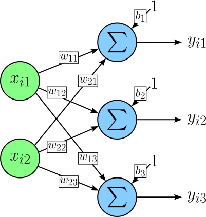
The operation each neuron performs is to compute the weighted sum of all inputs and then adding a bias, done during the forward pass (see below). If you check the figure above, a linear layer is fully described by a weight matrix $\mathbf{W}$ and a bias vector $\mathbf{b}$. For our example with a $2$-dimensional input and $3$ neurons in the linear layer, $\mathbf{W}$ is a $2\times 3$ matrix containing all the weights:

$$\large \mathbf{W} = \begin{bmatrix} w_{11} & w_{12} & w_{13}\\ w_{21} & w_{22} & w_{23} \end{bmatrix} \ \in \mathbb{R}^{2\times 3} $$

More generally, if $D$ is the dimensionality of the inputs (here: $D=2$) and $M$ is the number of neurons (here: $M = 3$), the weight matrix $\mathbf{W}$ has a shape of $D\times M$. Similarly, the bias vector $\mathbf{b}$ contains all $M$ bias values $\mathbf{b}_k$.

$$\large \mathbf{b} = \begin{bmatrix} b_{1} & b_{2} & b_{3}\\ \end{bmatrix} \ \in \mathbb{R}^{1\times 3} $$

Again, in general, the size of the bias vector $\mathbf{b}$ is $1\times M$.

Lastly, we also need to define an input for the linear layer. In line with the figure above, we assume $2$-dimensional inputs. Let's further assume a batch size of $2$, i.e., two $2$-dimensional inputs at the same time. This gives us a $2\times 2$ input matrix $\mathbf{X}$:

$$\large \mathbf{X} = \begin{bmatrix} x_{11} & x_{12}\\ x_{21} & x_{22} \end{bmatrix} \ \in \mathbb{R}^{2\times 2} $$

For an arbitrary input dimension size $D$ and number of individual input samples $N$ in the same batch, the size of the input matrix $\mathbf{X}$ is $N\times D$. Throughout this notebook, for all example computations, we assume $N=2$, $D=2$, and $M=3$ to keep things simple. However, all results are directly applicable to larger inputs (both $N$ and $D$) and larger linear layers in terms of the number of neurons $M$.

Forward Pass¶

In a neural network, the forward pass is the process of computing the output of the network for a given input. Starting from the input layer, data is passed sequentially through each layer, with each layer's output becoming the input to the next layer. The forward pass continues until the final layer produces the network's prediction or output. This output is then used to compute a loss $\mathcal{L}$ value by comparing it to the ground truth provided by the annotated training dataset. Importantly, the forward pass defines how information flows through the model and establishes the intermediate values that are later needed during the backward pass to compute gradients for learning.

The operation each neuron of a linear layer performs during the forward pass is to compute the weighted sum of the input features plus a bias. More concretely, for a single (i.e., unbatched) input vector $x_{i} \in \mathbb{R}^D$, the $k$-th neuron computes:

$$\large y_{ik} = \mathbf{w}_k^\top \mathbf{x}_{i} + b_k $$

where $\mathbf{x}_i = [x_{i1}, x_{i2}, \dots, x_{iD}]^\top$ is the input vector of size $D$, and $\mathbf{w}_k = [w_{1k}, w_{2k},\dots w_{Dk}]$ is the weight vector associated with that $k$-th neuron and $b_k$ is its bias. Each neuron therefore produces one scalar output that represents how strongly the input aligns with its learned weight vector, shifted by the bias.

In practice, we compute the forward pass for all neurons and with respect to all inputs in a batch in parallel. We can express this computation using the following matrix notations, each of the components we have already defined:

$$\large \mathbf{Y}\ = \mathbf{X}\mathbf{W} + \mathbf{b} $$

Note that the matrix product $\mathbf{XW}$ produces an output of shape $N \times D$, i.e., one output vector per input sample. Since the bias is defined per neuron and not per sample, it must be added to every row of this matrix. This is why broadcasting is needed. Broadcasting means that the bias vector $\mathbf{b}$ is conceptually replicated $N$ times, once for each sample in the batch, so that it can be added element-wise to $\mathbf{XW}$. In practice, no actual copying is required; instead, $\mathbf{b}$ is treated as if it had shape $N \times D$, allowing the addition to be carried out efficiently.

Let's have a look at the actual operations that are performed:

$$ \begin{align} \large \mathbf{Y}\ &\large= \mathbf{X}\mathbf{W} + \mathbf{b}\\[1em] &\large= \begin{bmatrix} x_{11} & x_{12}\\ x_{21} & x_{22} \end{bmatrix} \begin{bmatrix} w_{11} & w_{12} & w_{13}\\ w_{21} & w_{22} & w_{23} \end{bmatrix} + \begin{bmatrix} b_{1} & b_{2} & b_{3}\\ \end{bmatrix} \\[1em] &\large= \begin{bmatrix} x_{11}w_{11}+x_{12}w_{21}+b_{1} & x_{11}w_{12}+x_{12}w_{22}+b_{2} & x_{11}w_{13}+x_{12}w_{23}+b_{3}\\ x_{21}w_{11}+x_{22}w_{21}+b_{1} & x_{21}w_{12}+x_{22}w_{22}+b_{2} & x_{21}w_{13}+x_{22}w_{23}+b_{3} \end{bmatrix} \ \in \mathbb{R}^{2\times 3} \end{align} $$

By using $y_{ik}$ to denote output of the $k$-th neuron for the $i$-th input sample, we can get the following $N\times M$ (here: $2 \times 3$) output matrix $\mathbf{Y}$:

$$ \begin{align} \large \mathbf{Y}\ &\large= \begin{bmatrix} y_{11} & y_{12} & y_{13}\\ y_{21} & y_{22} & y_{23} \end{bmatrix} \ \in \mathbb{R}^{2\times 3} \end{align} $$

Assuming the linear layer is part of a larger neural network, the output matrix $\mathbf{Y}$ is then passed as the input to any subsequent input layer(s), until the last network layer returns the final output. During inference, the final output is then used to make predictions.

In contrast, during training the output of the last network layer is used to compute the loss $\mathcal{L}$ given the ground truth from the training data. Training the network now means to systematically adjust all network parameters, such as the weights and biases of a linear layer, and modify the output such that loss $\mathcal{L}$ decreases. For this, we need to compute the gradient of model parameters with respect to $\mathcal{L}$. So this is what we look at next.

Backward Pass¶

In a neural network, the process of computing gradients of the loss with respect to the model's parameters and intermediate activations (i.e., the outputs of previous layers) as called the backward pass. Starting from the loss at the output layer, gradients are propagated backward through the network using the chain rule of calculus. During the backward pass, each layer determines how much it contributed to the final error by computing gradients with respect to its weights, biases, and inputs. These gradients are then used by an optimization algorithm (such as gradient descent) to update the parameters, enabling the network to learn from data.

In the following, we assume that our linear layer is some layer in the network — that is; it received its input $\mathbf{X}$ as the output from a previous layer and passed its output $\mathbf{Y}$ to a subsequent layer. The latter assumes that during the backward pass through the linear layer, the upstream gradient $\frac{\partial \mathcal{L}}{\partial \mathbf{Y}}$ has been computed.

Since loss $\mathcal{L}$ is a scaler and $\mathbf{Y}$ is matrix of shape $N\times M$, the gradient $\frac{\partial \mathcal{L}}{\partial \mathbf{Y}}$ will also have a shape of $N\times M$, with each element of $\frac{\partial \mathcal{L}}{\partial \mathbf{Y}}$ being the derivative of $\mathcal{L}$ with respect to one element in $\mathbf{Y}$. In other words, $\frac{\partial \mathcal{L}}{\partial \mathbf{Y}}$ is the Jacobian matrix (or just Jacobian), i.e., the matrix of all first-order partial derivatives of a function with multiple inputs and multiple outputs. It measures the sensitivity of each output component with respect to each input component.

$$\large \frac{\partial\mathcal{L}}{\partial \mathbf{Y}} = \begin{bmatrix} \frac{\partial \mathcal{L}}{\partial y_{11}} & \frac{\partial \mathcal{L}}{\partial y_{12}} & \frac{\partial \mathcal{L}}{\partial y_{13}}\\ \frac{\partial \mathcal{L}}{\partial y_{12}} & \frac{\partial \mathcal{L}}{\partial y_{22}} & \frac{\partial \mathcal{L}}{\partial y_{23}} \end{bmatrix} $$

As part of the backward pass through the linear layer, our goals is now to compute the gradients $\frac{\partial \mathcal{L}}{\partial \mathbf{X}}$ (i.e., the downstream gradient passed to the previous layer according to the forward pass), as well as the gradients $\frac{\partial \mathcal{L}}{\partial \mathbf{W}}$ and $\frac{\partial \mathcal{L}}{\partial \mathbf{b}}$ to update all weights and biases based on the optimization method (e.g., gradient descent). By using the chain rule, we can calculate these gradients as follows:

$$\large \frac{\partial \mathcal{L}}{\partial \mathbf{X}} = \frac{\partial\mathbf{Y}}{\partial\mathbf{X}} \frac{\partial\mathcal{L}}{\partial\mathbf{Y}}\ , \qquad \frac{\partial \mathcal{L}}{\partial \mathbf{W}} = \frac{\partial\mathbf{Y}}{\partial\mathbf{W}} \frac{\partial\mathcal{L}}{\partial\mathbf{Y}}\ , \qquad \frac{\partial \mathcal{L}}{\partial \mathbf{b}} = \frac{\partial\mathbf{Y}}{\partial\mathbf{b}} \frac{\partial\mathcal{L}}{\partial\mathbf{Y}} $$

Since we got $\frac{\partial\mathcal{L}}{\partial\mathbf{Y}}$ as the upstream gradient from the subsequent layer, we now have to compute the gradients, i.e., the Jacobians, $\frac{\partial\mathbf{Y}}{\partial\mathbf{X}}$, $\frac{\partial\mathbf{Y}}{\partial\mathbf{W}}$, and $\frac{\partial\mathbf{Y}}{\partial\mathbf{b}}$.

Notice that the full Jacobian matrices would be extremely large as it contains the first-order partial derivatives for each outputs with respect to each input. For example, in the case of $\frac{\partial\mathbf{Y}}{\partial\mathbf{X}}$, since $\mathbf{Y}$ is of shape $N\times M$ and $\mathbf{X}$ is of shape $N\times D$, we have $N\cdot M$ outputs and $N\cdot D$ inputs. Thus the total number of elements in the Jacobian for $\frac{\partial\mathbf{Y}}{\partial\mathbf{X}}$ would be $N^2 \cdot N\cdot D$. Assuming some practical values of $N=64$ and $M=D=4096$, this would result in more than 68 million values and a memory footprint of 256 GB (assuming 32-bit floating point precision).

Fortunately, we can compute $\frac{\partial\mathbf{Y}}{\partial\mathbf{X}} \frac{\partial\mathcal{L}}{\partial\mathbf{Y}}$ (and the other gradients) without computing and storing the full Jacobian $\frac{\partial\mathcal{Y}}{\partial\mathbf{X}}$; as we will see next. The intuition is that a linear layer is composed of many independent dot products. Each dot product only "touches" a small subset of variables. The Jacobian simply encodes these dependency relationships, and because most variables do not interact, most entries are zero. Backpropagation (i.e., the backward pass) exploits this structure: instead of storing a huge sparse Jacobian, it directly computes how gradients flow through these local connections using matrix multiplications.

So, let's computed the three gradients $\frac{\partial \mathcal{L}}{\partial \mathbf{X}}$, $\frac{\partial \mathcal{L}}{\partial \mathbf{W}}$, and $\frac{\partial \mathcal{L}}{\partial \mathbf{b}}$ step by step.

Computing $\frac{\partial \mathcal{L}}{\partial \mathbf{X}}$¶

We start with $\frac{\partial \mathcal{L}}{\partial \mathbf{X}}$, which serves as the downstream gradient to be passed the previous layer to continue the backward pass. Although we do not know the values, we already know the shape the Jacobian $\frac{\partial \mathcal{L}}{\partial \mathbf{X}}$ must have. Again, since loss $\mathcal{L}$ is a scalar value, the shape of the Jacobian must be the as the one of $\mathbf{X}$:

$$\large \mathbf{X} = \begin{bmatrix} x_{11} & x_{12}\\ x_{21} & x_{22} \end{bmatrix} \quad \Longrightarrow \quad \frac{\partial \mathcal{L}}{\partial \mathbf{X}} = \begin{bmatrix} \frac{\partial\mathcal{L}}{\partial x_{11}} &\frac{\partial\mathcal{L}}{\partial x_{12}}\\ \frac{\partial\mathcal{L}}{\partial x_{21}} & \frac{\partial\mathcal{L}}{\partial x_{22}} \end{bmatrix} $$

Let's consider a single gradient, say, $\frac{\partial\mathcal{L}}{\partial x_{11}}$ and it is computed. Once we have this one, we can easily derive the remaining gradients in the Jacobian $\frac{\partial \mathcal{L}}{\partial \mathbf{X}}$. In principle, we computing $\frac{\partial\mathcal{L}}{\partial x_{11}}$, we must account for every path through which $x_{11}$ influences (or might influence) the loss $\mathcal{L}$. Since all outputs contribute independently, i.e.:

$x_{11} \rightarrow y_{11} \rightarrow \mathcal{L}$
$x_{11} \rightarrow y_{12} \rightarrow \mathcal{L}$
$x_{11} \rightarrow y_{13} \rightarrow \mathcal{L}$
$x_{11} \rightarrow y_{21} \rightarrow \mathcal{L}$
$x_{11} \rightarrow y_{22} \rightarrow \mathcal{L}$
$x_{11} \rightarrow y_{23} \rightarrow \mathcal{L}$

We have to add all these paths, because the loss aggregates all outputs. Thus, the gradient $\frac{\partial\mathcal{L}}{\partial x_{11}}$ is computed as the sum of all partial derivatives $\frac{\partial y_{ik}}{\partial x_{11}}$:

$$\large \frac{\partial \mathcal{L}}{\partial x_{11}} = \sum_{i=1}^N\sum_{k=1}^M \frac{\partial\mathcal{L}}{\partial y_{ik}}\frac{\partial y_{ik}}{\partial x_{11}} $$

However, if you think about it, we already know the same partial derivatives will be $0$. In fact, all $\frac{\partial y_{2k}}{\partial x_{11}}$ will be $0$ since the 1st input sample has no effect on the outputs with the 2nd sample. This means that we can simplify the formula by ignoring all terms that include the outputs for the 2nd and keep only the ones for the 1st sample, i.e., all $y_{1k}$. In short, we can drop the first sum and fix the value to $i=1$:

$$\large \frac{\partial \mathcal{L}}{\partial x_{11}} = \sum_{k=1}^M \frac{\partial\mathcal{L}}{\partial y_{1k}}\frac{\partial y_{1k}}{\partial x_{11}} $$

For clarity, let's expand the sum to show all individual terms.

$$\large \frac{\partial \mathcal{L}}{\partial x_{11}} = \frac{\partial\mathcal{L}}{\partial y_{11}}\frac{\partial y_{11}}{\partial x_{11}} + \frac{\partial\mathcal{L}}{\partial y_{12}}\frac{\partial y_{12}}{\partial x_{11}} + \frac{\partial\mathcal{L}}{\partial y_{13}}\frac{\partial y_{13}}{\partial x_{11}} $$

Again, we already have all values for $\frac{\partial\mathcal{L}}{\partial y_{11}}$, $\frac{\partial\mathcal{L}}{\partial y_{12}}$, and $ \frac{\partial\mathcal{L}}{\partial y_{13}}$ from the upstream gradient $\frac{\partial\mathcal{L}}{\partial\mathbf{Y}}$. To compute, $\frac{\partial y_{11}}{\partial x_{11}}$, $\frac{\partial y_{12}}{\partial x_{11}}$, and $\frac{\partial y_{13}}{\partial x_{11}}$, recall that the values for $y_{11}$, $y_{12}$, and $y_{13}$ are computed as follows:

$$ \begin{align} \large \mathbf{Y}\ &\large= \begin{bmatrix} y_{11} & y_{12} & y_{13}\\ y_{21} & y_{22} & y_{23} \end{bmatrix} = \large \begin{bmatrix} x_{11}w_{11}+x_{12}w_{21}+b_{1} & x_{11}w_{12}+x_{12}w_{22}+b_{2} & x_{11}w_{13}+x_{12}w_{23}+b_{3}\\ x_{21}w_{11}+x_{22}w_{21}+b_{1} & x_{21}w_{12}+x_{22}w_{22}+b_{2} & x_{21}w_{13}+x_{22}w_{23}+b_{3} \end{bmatrix} \end{align} $$

The three missing gradients are therefore:

$$ \begin{align} \large \frac{\partial y_{11}}{\partial x_{11}}\ &\large= \frac{\partial (x_{11}w_{11}+x_{12}w_{21}+b_{1})}{\partial x_{11}} = w_{11}\\[1em] \large \frac{\partial y_{12}}{\partial x_{11}}\ &\large= \frac{\partial (x_{11}w_{12}+x_{12}w_{22}+b_{2})}{\partial x_{11}} = w_{12}\\[1em] \large \frac{\partial y_{13}}{\partial x_{11}}\ &\large= \frac{\partial (x_{11}w_{13}+x_{12}w_{23}+b_{3})}{\partial x_{11}} = w_{13} \end{align} $$

We can no plug these value into our the expression for $\frac{\partial \mathcal{L}}{\partial x_{11}}$:

$$\large \frac{\partial \mathcal{L}}{\partial x_{11}} = \frac{\partial\mathcal{L}}{\partial y_{11}}w_{11} + \frac{\partial\mathcal{L}}{\partial y_{12}}w_{12} + \frac{\partial\mathcal{L}}{\partial y_{13}}w_{13} $$

Using the exact same steps, we can compute all for gradients in the Jacobian$ \frac{\partial \mathcal{L}}{\partial \mathbf{X}}$:

$$ \begin{align} \large\frac{\partial \mathcal{L}}{\partial x_{11}}\ &\large= \frac{\partial\mathcal{L}}{\partial y_{11}}w_{11} + \frac{\partial\mathcal{L}}{\partial y_{12}}w_{12} + \frac{\partial\mathcal{L}}{\partial y_{13}}w_{13}\\[1em] \large\frac{\partial \mathcal{L}}{\partial x_{12}}\ &\large= \frac{\partial\mathcal{L}}{\partial y_{11}}w_{21} + \frac{\partial\mathcal{L}}{\partial y_{12}}w_{22} + \frac{\partial\mathcal{L}}{\partial y_{13}}w_{23}\\[1em] \large\frac{\partial \mathcal{L}}{\partial x_{21}}\ &\large= \frac{\partial\mathcal{L}}{\partial y_{21}}w_{11} + \frac{\partial\mathcal{L}}{\partial y_{22}}w_{12} + \frac{\partial\mathcal{L}}{\partial y_{23}}w_{13}\\[1em] \large\frac{\partial \mathcal{L}}{\partial x_{22}}\ &\large= \frac{\partial\mathcal{L}}{\partial y_{21}}w_{21} + \frac{\partial\mathcal{L}}{\partial y_{22}}w_{22} + \frac{\partial\mathcal{L}}{\partial y_{23}}w_{23} \end{align} $$

We can take all for expressions and actually place them into the Jacobian $\frac{\partial \mathcal{L}}{\partial \mathbf{X}}$:

$$ \begin{align} \large\frac{\partial \mathcal{L}}{\partial \mathbf{X}}\ &\large= \begin{bmatrix} \frac{\partial\mathcal{L}}{\partial x_{11}} &\frac{\partial\mathcal{L}}{\partial x_{12}}\\ \frac{\partial\mathcal{L}}{\partial x_{21}} & \frac{\partial\mathcal{L}}{\partial x_{22}} \end{bmatrix}\\[1em] &\large = \begin{bmatrix} \frac{\partial\mathcal{L}}{\partial y_{11}}w_{11} + \frac{\partial\mathcal{L}}{\partial y_{12}}w_{12} + \frac{\partial\mathcal{L}}{\partial y_{13}}w_{13} & \frac{\partial\mathcal{L}}{\partial y_{11}}w_{21} + \frac{\partial\mathcal{L}}{\partial y_{12}}w_{22} + \frac{\partial\mathcal{L}}{\partial y_{13}}w_{23}\\ \frac{\partial\mathcal{L}}{\partial y_{21}}w_{11} + \frac{\partial\mathcal{L}}{\partial y_{22}}w_{12} + \frac{\partial\mathcal{L}}{\partial y_{23}}w_{13} & \frac{\partial\mathcal{L}}{\partial y_{21}}w_{21} + \frac{\partial\mathcal{L}}{\partial y_{22}}w_{22} + \frac{\partial\mathcal{L}}{\partial y_{23}}w_{23} \end{bmatrix} \end{align} $$

As the last step — just by looking at it hard enough — we can decompise $\frac{\partial \mathcal{L}}{\partial \mathbf{X}}$ into a product of the upstream gradient $\frac{\partial \mathcal{L}}{\partial \mathbf{Y}}$ and the transpose of the weight matrix $\mathbf{W}$:

$$ \begin{align} \large\frac{\partial \mathcal{L}}{\partial \mathbf{X}}\ &\large= \begin{bmatrix} \frac{\partial\mathcal{L}}{\partial y_{11}} & \frac{\partial\mathcal{L}}{\partial y_{12}} & \frac{\partial\mathcal{L}}{\partial y_{13}}\\ \frac{\partial\mathcal{L}}{\partial y_{21}} & \frac{\partial\mathcal{L}}{\partial y_{22}} & \frac{\partial\mathcal{L}}{\partial y_{23}} \end{bmatrix} \begin{bmatrix} w_{11} & w_{21} \\ w_{12} & w_{22} \\ w_{13} & w_{23} \\ \end{bmatrix}\\[1em] &\large = \frac{\partial \mathcal{L}}{\partial \mathbf{Y}}\mathbf{W}^\top \end{align} $$

In short, we can compute the gradients $\large\frac{\partial \mathcal{L}}{\partial \mathbf{X}}$ simply by multiplying the upstream gradient $\frac{\partial \mathcal{L}}{\partial \mathbf{Y}}$ from the subsequent layer (with respect to the forward pass) and the transpose of the weight matrix $\mathbf{W}$ of the linear layer.

Side note: Recall that the full Jacobian matrix $\frac{\partial\mathbf{Y}}{\partial\mathbf{X}}$ would have $N^2 \cdot N\cdot D$ elements. More specifically, $\frac{\partial\mathbf{Y}}{\partial\mathbf{X}}$ would have the following block-diagonal structure, where each block corresponds to one sample in the batch. There are $N$ diagonal blocks, one per input sample, and each block has shape $M\times D$ and is exactly the weight matrix $\mathbf{W}^\top$. All off-diagonal blocks are zero matrices.

$$\large \frac{\partial\mathbf{Y}}{\partial\mathbf{X}} = \begin{bmatrix} \mathbf{W}^\top & 0 & \cdots & 0 \\ 0 & \mathbf{W}^\top & \cdots & 0 \\ \vdots & \vdots & \ddots & \vdots \\ 0 & 0 & \cdots & \mathbf{W}^\top \end{bmatrix} $$

This structure occurs because the outputs from one sample depend only on the inputs from that sample sample (n), and never on other samples in the batch. Therefore, derivatives across different samples are zero. Within each sample, each output neuron is a linear combination of the input features, encoded by $\mathbf{W}^\top$. This highly sparse, block-diagonal structure explains both why the full Jacobian contains many zeros and why we can replace it with a simple matrix multiplication in the backward pass.

Computing $\frac{\partial \mathcal{L}}{\partial \mathbf{W}}$¶

Having gone trough all steps to compute $\frac{\partial \mathcal{L}}{\partial \mathbf{X}}$, we can now compute $\frac{\partial \mathcal{L}}{\partial \mathbf{W}}$ basically the same, i.e., perform the same core steps. Once again, we already know that the shape of $\frac{\partial \mathcal{L}}{\partial \mathbf{W}}$ must be the same as $\mathbf{X}$ as loss $\mathcal{L}$ is a scalar values:

$$\large \mathbf{X} = \begin{bmatrix} w_{11} & w_{12} & w_{13}\\ w_{21} & w_{22} & w_{23} \end{bmatrix} \quad \Longrightarrow \quad \frac{\partial \mathcal{L}}{\partial \mathbf{W}} = \begin{bmatrix} \frac{\partial\mathcal{L}}{\partial w_{11}} & \frac{\partial\mathcal{L}}{\partial w_{12}} & \frac{\partial\mathcal{L}}{\partial w_{13}}\\ \frac{\partial\mathcal{L}}{\partial w_{21}} & \frac{\partial\mathcal{L}}{\partial w_{22}} & \frac{\partial\mathcal{L}}{\partial w_{23}} \end{bmatrix} $$

Focusing on a single element of this Jacobian matrix, say, $\frac{\partial \mathcal{L}}{\partial w_{11}}$, we have to consider all possible paths how $w_{11}$ maye have affected $\mathcal{L}$ through any output $y_{ik}$ using the chain rule. Thus, $\frac{\partial \mathcal{L}}{\partial w_{11}}$ is the sum of all these paths.

$$\large \frac{\partial \mathcal{L}}{\partial w_{11}} = \sum_{i=1}^N\sum_{k=1}^M \frac{\partial\mathcal{L}}{\partial y_{ik}}\frac{\partial y_{ik}}{\partial w_{11}} $$

But again, we can first simplify this expression since we already know that some partial derivatives $\frac{\partial y_{ik}}{\partial w_{11}}$ will be $0$. Here, since $w_{11}$ can only affect the 1st neuron (i.e., k=1), only the partial derivatives $\frac{\partial y_{i1}}{\partial w_{11}}$ can yield non-zero values. This means that we can get rid of the 2nd sum and fix the value of $k$ to $1$:

$$\large \frac{\partial \mathcal{L}}{\partial w_{11}} = \sum_{i=1}^N \frac{\partial\mathcal{L}}{\partial y_{i1}}\frac{\partial y_{i1}}{\partial w_{11}} $$

In short, we only sum with respect to the number of samples in the input batch. As before, let's expand the sum just for clarity.

$$\large \frac{\partial \mathcal{L}}{\partial w_{11}} = \frac{\partial\mathcal{L}}{\partial y_{11}}\frac{\partial y_{11}}{\partial w_{11}} + \frac{\partial\mathcal{L}}{\partial y_{21}}\frac{\partial y_{21}}{\partial w_{11}} $$

To compute the two partial derivates $\frac{\partial y_{11}}{\partial w_{11}}$ and $\frac{\partial y_{21}}{\partial w_{21}}$, it is useful to look at the definition of $\mathbf{Y}$.

Given this, the solutions for the two partial derivatives are as follows:

$$ \begin{align} \large \frac{\partial y_{11}}{\partial w_{11}}\ &\large= \frac{\partial (x_{11}w_{11}+x_{12}w_{21}+b_{1})}{\partial w_{11}} = x_{11}\\[1em] \large \frac{\partial y_{21}}{\partial w_{11}}\ &\large= \frac{\partial (x_{21}w_{11}+x_{22}w_{21}+b_{1})}{\partial w_{11}} = x_{21} \end{align} $$

Performing these steps for all $6$ gradients $\frac{\partial \mathcal{L}}{\partial w_{ik}}$ will gives us the following $6$ expressions:

$$ \begin{align} \large\frac{\partial \mathcal{L}}{\partial w_{11}}\ &\large= \frac{\partial\mathcal{L}}{\partial y_{11}}x_{11} + \frac{\partial\mathcal{L}}{\partial y_{21}}x_{21}\\[1em] \large\frac{\partial \mathcal{L}}{\partial w_{12}}\ &\large= \frac{\partial\mathcal{L}}{\partial y_{12}}x_{11} + \frac{\partial\mathcal{L}}{\partial y_{22}}x_{21}\\[1em] \large\frac{\partial \mathcal{L}}{\partial w_{13}}\ &\large= \frac{\partial\mathcal{L}}{\partial y_{13}}x_{11} + \frac{\partial\mathcal{L}}{\partial y_{23}}x_{21}\\[1em] \large\frac{\partial \mathcal{L}}{\partial w_{21}}\ &\large= \frac{\partial\mathcal{L}}{\partial y_{11}}x_{12} + \frac{\partial\mathcal{L}}{\partial y_{21}}x_{22}\\[1em] \large\frac{\partial \mathcal{L}}{\partial w_{22}}\ &\large= \frac{\partial\mathcal{L}}{\partial y_{12}}x_{12} + \frac{\partial\mathcal{L}}{\partial y_{22}}x_{22}\\[1em] \large\frac{\partial \mathcal{L}}{\partial w_{23}}\ &\large= \frac{\partial\mathcal{L}}{\partial y_{13}}x_{12} + \frac{\partial\mathcal{L}}{\partial y_{23}}x_{22} \end{align} $$

We can now rewrite the $\large\frac{\partial \mathcal{L}}{\partial \mathbf{W}}$ by replacing all $\frac{\partial\mathcal{L}}{\partial w_{ik}}$ with their corresponding solutions.

$$ \begin{align} \large\frac{\partial \mathcal{L}}{\partial \mathbf{W}}\ &\large= \begin{bmatrix} \frac{\partial\mathcal{L}}{\partial w_{11}} & \frac{\partial\mathcal{L}}{\partial w_{12}} & \frac{\partial\mathcal{L}}{\partial w_{13}}\\ \frac{\partial\mathcal{L}}{\partial w_{21}} & \frac{\partial\mathcal{L}}{\partial w_{22}} & \frac{\partial\mathcal{L}}{\partial w_{23}} \end{bmatrix}\\[1em] &\large = \begin{bmatrix} \frac{\partial\mathcal{L}}{\partial y_{11}}x_{11} + \frac{\partial\mathcal{L}}{\partial y_{21}}x_{21} & \frac{\partial\mathcal{L}}{\partial y_{12}}x_{11} + \frac{\partial\mathcal{L}}{\partial y_{22}}x_{21} & \frac{\partial\mathcal{L}}{\partial y_{13}}x_{11} + \frac{\partial\mathcal{L}}{\partial y_{23}}x_{21}\\ \frac{\partial\mathcal{L}}{\partial y_{11}}x_{12} + \frac{\partial\mathcal{L}}{\partial y_{21}}x_{22} & \frac{\partial\mathcal{L}}{\partial y_{12}}x_{12} + \frac{\partial\mathcal{L}}{\partial y_{22}}x_{22} & \frac{\partial\mathcal{L}}{\partial y_{13}}x_{12} + \frac{\partial\mathcal{L}}{\partial y_{23}}x_{22} \end{bmatrix} \end{align} $$

Last, we can again decompose this Jacobian into a product of two matrices, the transpose of input matrix $\mathbf{X}$ and the upstream gradient $\frac{\partial\mathcal{L}}{\partial w_{11}}$:

$$ \begin{align} \large\frac{\partial \mathcal{L}}{\partial \mathbf{W}}\ &\large= \begin{bmatrix} x_{11} & x_{21} \\ x_{12} & x_{22} \end{bmatrix} \begin{bmatrix} \frac{\partial\mathcal{L}}{\partial y_{11}} & \frac{\partial\mathcal{L}}{\partial y_{12}} & \frac{\partial\mathcal{L}}{\partial y_{13}}\\ \frac{\partial\mathcal{L}}{\partial y_{21}} & \frac{\partial\mathcal{L}}{\partial y_{22}} & \frac{\partial\mathcal{L}}{\partial y_{23}} \end{bmatrix}\\[1em] &\large = \mathbf{X}^\top \frac{\partial\mathcal{L}}{\partial\mathbf{Y}} \end{align} $$

This solution shows that the linear layer needs to store $\mathbf{X}$ for the backward pass. In other words, the memory footprint of a linear layer — at least during training — is not just determined by its weights and biases but also by its input from the previous layer. As the shape of input matrix $\mathbf{X}$ is $N\times D$, it is easy to see that the batch size $N$ becomes an important factor affecting the overall memory requirements for training a neural network.

Side note: Notice that we once more avoided to compute the full Jacobian matrix $\frac{\partial \mathcal{L}}{\partial \mathbf{W}}$ which has the following form:

$$\large \frac{\partial \mathbf{Y}}{\partial \mathbf{W}} = \begin{bmatrix} X & 0 & \cdots & 0 \\ 0 & X & \cdots & 0 \\ \vdots & \vdots & \ddots & \vdots \\ 0 & 0 & \cdots & X \end{bmatrix} $$

However, like for $\frac{\partial \mathcal{L}}{\partial \mathbf{W}}$, the block-diagonal structure and each block corresponding to the input matrix $\mathbf{X}$ allows avoiding the computation of the full Jacobian matrix as the "simply" solution for $\frac{\partial \mathbf{Y}}{\partial \mathbf{W}}$ yields the same result.

Computing $\frac{\partial \mathcal{L}}{\partial \mathbf{b}}$¶

The last remaining gradient we need to compute is $\frac{\partial \mathcal{L}}{\partial \mathbf{b}}$, but the steps to accomplish this are the same. Knowing the shape of bias vector $\mathbf{b}$, we also know the shape of the Jacobian matrix $\frac{\partial \mathcal{L}}{\partial \mathbf{b}}$.

$$\large \mathbf{b} = \begin{bmatrix} b_{1} & b_{2} & b_{3} \end{bmatrix} \quad \Longrightarrow \quad \frac{\partial \mathcal{L}}{\partial \mathbf{b}} = \begin{bmatrix} \frac{\partial\mathcal{L}}{\partial b_{1}} & \frac{\partial\mathcal{L}}{\partial b_{2}} & \frac{\partial\mathcal{L}}{\partial b_{3}} \end{bmatrix} $$

Let's consider an individual entry, say, $\frac{\partial\mathcal{L}}{\partial b_{1}}$. Its value, in principle, depends on all paths $b_1$ may affect the value of $\mathcal{L}$, which can be determined using the chain rule. Thus, $\frac{\partial\mathcal{L}}{\partial b_{1}}$ is the sum of all these possible paths.

$$\large \frac{\partial \mathcal{L}}{\partial b_{1}} = \sum_{i=1}^N\sum_{j=1}^M \frac{\partial\mathcal{L}}{\partial y_{ij}}\frac{\partial y_{ij}}{\partial b_{1}} $$

Like for $\frac{\partial \mathcal{L}}{\partial w_{11}}$, we know that $b_1$ can only affect the output values $y_{i1}$ of the 1st neuron. This allows us to simplify the expression by removing the 2nd sum, fix the value of $k$ to $1$, and sum only with respect to the number of samples $N$ in the input batch.

$$\large \frac{\partial \mathcal{L}}{\partial b_{1}} = \sum_{i=1}^{N} \frac{\partial\mathcal{L}}{\partial y_{i1}}\frac{\partial y_{i1}}{\partial b_{1}} $$

By expanding this sum, we can quickly see which partial derivatives we need to compute.

$$\large \frac{\partial \mathcal{L}}{\partial b_{1}} = \frac{\partial\mathcal{L}}{\partial y_{11}}\frac{\partial y_{11}}{\partial b_{1}} + \frac{\partial\mathcal{L}}{\partial y_{21}}\frac{\partial y_{21}}{\partial b_{1}} $$

To compute the two partial derivatives $\frac{\partial y_{11}}{\partial b_{1}}$ and $\frac{\partial y_{21}}{\partial b_{1}}$ it helps again to look at the definition of $\mathbf{Y}$.

Since $b_1$ appears in the expressions for $y_{11}$ and $y_{21}$ only as an individual term of the sums, the partial derivatives simply evaluate to $1$.

$$ \begin{align} \large \frac{\partial y_{11}}{\partial b_{1}}\ &\large= \frac{\partial (x_{11}w_{11}+x_{12}w_{21}+b_{1})}{\partial b_{1}} = 1\\[1em] \large \frac{\partial y_{21}}{\partial b_{1}}\ &\large= \frac{\partial (x_{21}w_{11}+x_{22}w_{21}+b_{1})}{\partial b_{1}} = 1 \end{align} $$

Performing these steps for all $\frac{\partial \mathcal{L}}{\partial b_{1}}$, and all partial derivatives $\frac{\partial y_{ik}}{\partial b_{k}}$ being $1$, we get the follwing three solutions:

$$ \begin{align} \large\frac{\partial \mathcal{L}}{\partial b_{1}}\ &\large= \frac{\partial\mathcal{L}}{\partial y_{11}}+ \frac{\partial\mathcal{L}}{\partial y_{21}}\\[1em] \large\frac{\partial \mathcal{L}}{\partial b_{2}}\ &\large= \frac{\partial\mathcal{L}}{\partial y_{12}} + \frac{\partial\mathcal{L}}{\partial y_{22}}\\[1em] \large\frac{\partial \mathcal{L}}{\partial b_{3}}\ &\large= \frac{\partial\mathcal{L}}{\partial y_{13}} + \frac{\partial\mathcal{L}}{\partial y_{23}} \end{align} $$

Using these solutions, we can rewrite the Jacobian matrix $\frac{\partial \mathcal{L}}{\partial \mathbf{b}}$ as:

$$ \begin{align} \large\frac{\partial \mathcal{L}}{\partial \mathbf{b}}\ &\large= \begin{bmatrix} \frac{\partial\mathcal{L}}{\partial b_{1}} & \frac{\partial\mathcal{L}}{\partial b_{2}} & \frac{\partial\mathcal{L}}{\partial b_{3}} \end{bmatrix}\\[1em] &\large = \begin{bmatrix} \frac{\partial\mathcal{L}}{\partial y_{11}} + \frac{\partial\mathcal{L}}{\partial y_{21}} & \frac{\partial\mathcal{L}}{\partial y_{12}} + \frac{\partial\mathcal{L}}{\partial y_{22}} & \frac{\partial\mathcal{L}}{\partial y_{13}} + \frac{\partial\mathcal{L}}{\partial y_{23}} \end{bmatrix} \end{align} $$

If you look closely, this solution is simply the row-wise sum of the upstream gradient $\frac{\partial\mathcal{L}}{\partial\mathbf{Y}}$. And in fact, when implementing the computation $\frac{\partial \mathcal{L}}{\partial \mathbf{b}}$ we typically just sum up all the rows of the upstream gradient. However, in principle we can once more decompose the Jacobian matrix $\frac{\partial \mathcal{L}}{\partial \mathbf{b}}$ into a product of two matrices where one of them is the upstream gradient $\frac{\partial\mathcal{L}}{\partial\mathbf{Y}}$:

$$ \begin{align} \large\frac{\partial \mathcal{L}}{\partial \mathbf{b}}\ &\large= \begin{bmatrix} 1 & 1 \end{bmatrix} \begin{bmatrix} \frac{\partial\mathcal{L}}{\partial y_{11}} & \frac{\partial\mathcal{L}}{\partial y_{12}} & \frac{\partial\mathcal{L}}{\partial y_{13}}\\ \frac{\partial\mathcal{L}}{\partial y_{21}} & \frac{\partial\mathcal{L}}{\partial y_{22}} & \frac{\partial\mathcal{L}}{\partial y_{23}} \end{bmatrix}\\[1em] &\large = \begin{bmatrix} 1 & 1 \end{bmatrix} \frac{\partial\mathcal{L}}{\partial\mathbf{Y}} \end{align} $$

In general, the matrix containing all $1$s will have a shape of $1\times N$.

This means we can now compute all three required gradients for the backward pass through a linear layer. Despite the rather tedious math, the final solutions are in fact very simple and arguably intuitive given the basic rules of backpropagation — although this might not be obvious from the outset, so it is better to go through the math. Summing up, these are the solutions for our $3$ gradients we need to compute:

$$ \large \frac{\partial \mathcal{L}}{\partial \mathbf{X}} = \frac{\partial \mathcal{L}}{\partial \mathbf{Y}}\mathbf{W}^\top\ , \qquad \frac{\partial \mathcal{L}}{\partial \mathbf{W}} = \mathbf{X}^\top \frac{\partial\mathcal{L}}{\partial\mathbf{Y}}\ , \qquad \frac{\partial \mathcal{L}}{\partial \mathbf{b}} = \begin{bmatrix} 1 & 1 & \dots & 1 \end{bmatrix} \frac{\partial\mathcal{L}}{\partial\mathbf{Y}} $$

Again, in practice, we typically do not compute the gradient $\frac{\partial \mathcal{L}}{\partial \mathbf{b}}$ as a product of these two matrices. Since this product yields the same result as simply adding all rows of the upstream gradient $\frac{\partial\mathcal{L}}{\partial\mathbf{Y}}$, the row-wise summation is typically easier and more efficient to implement.

Worked Example & Implementation¶

So far, we only worked with variables to find the general solutions for all the required gradients to perform the backward pass through a linear layer. So at the end, let's go through a simple example using some values and perform all the involved computations. In the following, show both the matrix expressions as well as the Python code using NumPy.

Data Definitions¶

We first need some example values for input matrix $\mathbf{X}$, weight matrix $\mathbf{W}$, and bias vector $\mathbf{b}$. Let's assume the same values for the number of samples in the input batch ($N=2$), for the dimensionality of the input ($D=2$), and the number of neurons ($M=3$) as we used throughout the notebook; see the illustration of a small linear layer at the top. And since we do not really care about the actual result, we can use some simple values to define two matrices and the vector.

$$\large \mathbf{X} = \begin{bmatrix} 0.1 & 0.2\\ 0.3 & 0.4 \end{bmatrix}\ ,\qquad \mathbf{W} = \begin{bmatrix} 0.1 & 0.2 & 0.3\\ 0.4 & 0.5 & 0.6 \end{bmatrix}\ ,\qquad \mathbf{b} = \begin{bmatrix} 0.1 & 0.2 & 0.3 \end{bmatrix} $$

For performing all computations using NumPy, we also need to define the data as NumPy arrays.

In [2]:

X = np.asarray([ [ 0.1, 0.2 ], [ 0.3, 0.4] ])
W = np.asarray([ [ 0.1, 0.2, 0.3 ], [ 0.4, 0.5, 0.6] ])
b = np.asarray([ [ 0.1, 0.2, 0.3 ] ])

So far, we have all the example data needed to perform the formward pass. For the backward pass, we also need the upstream gradient $\frac{\partial\mathcal{L}}{\partial\mathbf{Y}}$. Again, we do not really care about the result, so let's use some simple values to define the upstream gradient as well.

$$\large \frac{\partial\mathcal{L}}{\partial\mathbf{Y}} = \begin{bmatrix} 0.2 & 0.3 & 0.4\\ 0.5 & 0.6 & 0.7 \end{bmatrix} $$

Of course, we also need its representation as a NumPy array.

In [3]:

dY = np.asarray([ [ 0.2, 0.3, 0.4 ], [ 0.5, 0.6, 0.7] ])

Forward Pass¶

We saw that each neuron of a linear layer performs a weighted sum of the inputs and then adds a bias term. Doing this for all neurons in parallel given a batched input gave us the expression $\mathbf{Y} = \mathbf{X}\mathbf{W} + \mathbf{b}$ to compute the output of a linear layer is part of the forwards pass through a neural network. We can now replace the variable with our simple generated data to compute the output for example.

$$ \begin{align} \large \mathbf{Y}\ &\large= \mathbf{X}\mathbf{W} + \mathbf{b}\\[1em] &\large= \begin{bmatrix} 0.1 & 0.2\\ 0.3 & 0.4 \end{bmatrix} \begin{bmatrix} 0.1 & 0.2 & 0.3\\ 0.4 & 0.5 & 0.6 \end{bmatrix} + \begin{bmatrix} 0.1 & 0.2 & 0.3\\ \end{bmatrix} \\[1em] &\large= \begin{bmatrix} 0.09 & 0.12 & 0.15\\ 0.19 & 0.26 & 0.33\\ \end{bmatrix} + \begin{bmatrix} 0.1 & 0.2 & 0.3\\ \end{bmatrix} \\[1em] &\large= \begin{bmatrix} 0.19 & 0.32 & 0.45\\ 0.29 & 0.46 & 0.63\\ \end{bmatrix} \end{align} $$

Again, keep in mind that adding the bias vector $\mathbf{b}$ to the matrix $\mathbf{XW}$ relies on the concept of broadcasting, so that the bias vector is added to each row of the matrix. NumPy performs broadcasting under the hood as long as the shapes/dimensions of the involved arrays work out; which they do here, of course. In the code cell, below we implement the forwards pass using NumPy.

In [4]:

Y = X @ W + b

print(f"Shape of output Y: {Y.shape}\n")
print(f"Output Y:\n{Y}")

Shape of output Y: (2, 3)

Output Y:
[[0.19 0.32 0.45]
 [0.29 0.46 0.63]]

Note that in NumPy, the @ operator is syntactic sugar for matrix multiplication, introduced to clearly distinguish linear algebra operations from element-wise multiplication (*). When applied to arrays, A @ B follows standard linear algebra rules: for 2-D arrays it performs matrix–matrix multiplication, for 1-D arrays it computes inner products or matrix–vector products depending on the operands, and for higher-dimensional arrays it applies batched matrix multiplication over the leading dimensions using broadcasting. Under the hood, @ is equivalent to calling np.matmul(A, B), ensuring shape-aware multiplication that aligns with mathematical notation used in neural networks and other numerical computing tasks.

Backward Pass¶

Using our exampla data for the upstream gradient $\frac{\partial \mathcal{L}}{\partial \mathbf{Y}}$, we can compute all three required gradients as part for the backward pass. Let's start with $\frac{\partial \mathcal{L}}{\partial \mathbf{X}}$ by plugging in example our values into the definition for the gradient.

$$ \begin{align} \large\frac{\partial \mathcal{L}}{\partial \mathbf{X}}\ &\large= \frac{\partial \mathcal{L}}{\partial \mathbf{Y}}\mathbf{W}^\top\\[0.5em] &\large = \begin{bmatrix} 0.2 & 0.3 & 0.4\\ 0.5 & 0.6 & 0.7 \end{bmatrix} \begin{bmatrix} 0.1 & 0.4 \\ 0.2 & 0.5 \\ 0.3 & 0.6 \end{bmatrix}\\[0.5em] &\large = \begin{bmatrix} 0.20 & 0.47 \\ 0.38 & 0.92 \end{bmatrix} \end{align} $$

The equivalent NumPy code for this computation is shown in the code cell below.

In [5]:

dX = dY @ W.T

print(f"Shape of gradient dX: {dX.shape}\n")
print(f"Gradient dX:\n{dX}")

Shape of gradient dX: (2, 2)

Gradient dX:
[[0.2  0.47]
 [0.38 0.92]]

Next, we compute the gradient $\frac{\partial \mathcal{L}}{\partial \mathbf{W}}$ the same way. First showing the involved matrix operations...

$$ \begin{align} \large\frac{\partial \mathcal{L}}{\partial \mathbf{W}}\ &\large = \mathbf{X}^\top \frac{\partial\mathcal{L}}{\partial\mathbf{Y}}\\[0.5em] &\large = \begin{bmatrix} 0.1 & 0.3 \\ 0.2 & 0.4 \end{bmatrix} \begin{bmatrix} 0.2 & 0.3 & 0.4\\ 0.5 & 0.6 & 0.7 \end{bmatrix}\\[0.5em] &\large = \begin{bmatrix} 0.17 & 0.21 & 0.25\\ 0.24 & 0.30 & 0.36 \end{bmatrix} \end{align} $$

...and the corresponding Python code using NumPy.

In [6]:

dW = X.T @ dY

print(dW)

[[0.17 0.21 0.25]
 [0.24 0.3  0.36]]

Now only the gradient $\frac{\partial \mathcal{L}}{\partial \mathbf{b}}$ is left. As before, let's first look at the involved operations by plugging in the example values into our expression for the gradient.

$$ \begin{align} \large\frac{\partial \mathcal{L}}{\partial \mathbf{b}}\ &\large= \begin{bmatrix} 1 & 1 \end{bmatrix} \frac{\partial\mathcal{L}}{\partial\mathbf{Y}}\\[1em] &\large= \begin{bmatrix} 1 & 1 \end{bmatrix} \begin{bmatrix} 0.2 & 0.3 & 0.4\\ 0.5 & 0.6 & 0.7 \end{bmatrix}\\[0.5em] &\large = \begin{bmatrix} 0.7 & 0.9 & 1.1 \end{bmatrix} \end{align} $$

With respect to implementing this operation using NumPy, we actually have two main choices. For one, we can directly implement the computation in terms of a matrix multiplication as shown above.

In [7]:

db = np.asarray([1, 1]) @ dY

print(f"Shape of gradient db: {db.shape}\n")
print(f"Gradient db:\n{db}")

Shape of gradient db: (3,)

Gradient db:
[0.7 0.9 1.1]

However, we already know this matrix multiplication yields the same result as summing up all rows of the upstream gradient $\frac{\partial\mathcal{L}}{\partial\mathbf{Y}}$. Thus, instead of perform a matrix multiplication, we can use NumPy's built-on method sum() method with axis=0 to sum all all values with respect to axis/dimension $0$ which refers to the rows in case of a matrix, which we have here. The code cell below shows the corresponding code.

In [8]:

db = dY.sum(axis=0)

print(f"Shape of gradient db: {db.shape}\n")
print(f"Gradient db:\n{db}")

Shape of gradient db: (3,)

Gradient db:
[0.7 0.9 1.1]

Obviously, both approaches to compute $\frac{\partial \mathcal{L}}{\partial \mathbf{b}}$ yield the same result.

With this, we have completed the backward pass through the linear layer. With $\frac{\partial \mathcal{L}}{\partial \mathbf{W}}$ and $\frac{\partial \mathcal{L}}{\partial \mathbf{b}}$, we have the gradients to update the weights and biases of the linear layer, and with $\frac{\partial \mathcal{L}}{\partial \mathbf{X}}$ we have the downstream gradient to be passed to the previous layer to continue the backward words. Once again, appreciate how straightforward all computations are when using NumPy as we can directly implement the simple expressions for each gradient using very simple code.

Basic Linear Layer Class¶

In deep learning frameworks such as PyTorch or Tensorflow, layers are typically implemented as classes with explicit forward() and backward() methods because this structure mirrors both the mathematical definition of the layer and the way neural networks are trained. In case of a linear layer, the forward() method encapsulates the computation $\mathbf{Y} = \mathbf{X}\mathbf{W} + \mathbf{b}$, producing outputs from inputs, while the backward() method is responsible for computing gradients with respect to the inputs and parameters. Grouping these operations inside a single class makes the layer a self-contained computational unit that can be easily composed with other layers to form a full network, reflecting the modular nature of neural network architectures.

Crucially, the class must also store all intermediate data required for the backward pass, such as the input $\matrix{X}$ from the forward computation. During training, gradients flow backward through the network, and computing the gradient $\frac{\partial \mathcal{L}}{\partial \mathbf{W}}$ depends directly on values seen in the forward pass. By caching this information inside the layer object, the backward method can compute gradients efficiently without recomputing the forward pass or constructing large Jacobian matrices. This design not only improves computational efficiency but also makes the implementation closely align with the principles of backpropagation used in modern deep learning frameworks.

The code cell below shows the class Linear which represents a basic implementation of a linear layer. All the computations done in the forward() and backward() method, we have already seen above when computing the output and all gradients individually. The only additional consideration is the initialization of the weights $\mathbf{W}$ and biases $\mathbf{b}$.

In [9]:

class Linear:
    
    def __init__(self, in_features, out_features):
        # Weight initialization (simple Gaussian)
        self.W = np.random.randn(in_features, out_features) * 0.01
        self.b = np.zeros(out_features)

        # Gradients
        self.dW = np.zeros_like(self.W)
        self.db = np.zeros_like(self.b)

        # Cache for backward pass
        self.X = None

    def forward(self, X):
        self.X = X
        return X @ self.W + self.b

    def backward(self, dY):
        self.dW = self.X.T @ dY  # Gradient w.r.t. weights
        self.db = dY.sum(axis=0) # Gradient w.r.t. bias
        return dY @ self.W.T     # Gradient w.r.t. input

Well, let's create an instance of the class Linear with $D=2$ (in_features=2) amd $M=3$ (out_features=3) to match our small running example of a linear layer with $3$ neurons, receiving 2-dimensional data as inputs. To ensure the same result as before, we also have to "overwrite" the randomly initialized weights as well as the biases with the values from our example data.

In [10]:

linear = Linear(2, 3)

# Overwrite random weights and biases with example data
linear.W = W
linear.b = b

To compute the output $\mathbf{Y}$, we only need to call the forward() method and pass the input matrix $\mathbf{X}$ to the method.

In [11]:

Y = linear.forward(X)

print(f"Shape of output Y: {Y.shape}\n")
print(f"Output Y:\n{Y}")

Shape of output Y: (2, 3)

Output Y:
[[0.19 0.32 0.45]
 [0.29 0.46 0.63]]

With the backward() method and given the upstream gradient dY, we can compute the gradients dX, dW, and db. Note that in this particular implementation of the linear layer, the backward() method only returns downstream gradient dX so it can be passed to the previous layers as its upstream gradient. The gradients with respect to the weights and biases are specific to the layer and are therefore stored as member variables of the class.

In [12]:

dX = linear.backward(dY)

print(f"Shape of gradient dX: {Y.shape}\n")
print(f"Gradient dX:\n{dX}")

Shape of gradient dX: (2, 3)

Gradient dX:
[[0.2  0.47]
 [0.38 0.92]]

Of course, the return values of both the forward() and backward() method should match the result we got when computing the output and all gradients "manually".

Summary¶

This notebook provided a detailed, end-to-end treatment of the linear layer, starting from its mathematical definition and building up to a full understanding of how it is implemented in practice. We carefully derived the forward pass, $\mathbf{Y} = \mathbf{X}\mathbf{W} + \mathbf{b}$, emphasizing the role of matrix multiplication, batching, and bias broadcasting, and showed how this compact formulation naturally aligns with efficient numerical computation in NumPy and modern deep learning frameworks.

A central focus of the notebook was the backward pass and the mathematics required for efficient backpropagation. Rather than constructing large and mostly sparse Jacobian matrices explicitly, we derived the required gradients using matrix calculus and intuition about how outputs depend on inputs and parameters. This led to the familiar and efficient gradient expressions $\frac{\partial \mathcal{L}}{\partial \mathbf{X}} = \frac{\partial \mathcal{L}}{\partial \mathbf{Y}}\mathbf{W}^\top$, $\frac{\partial \mathcal{L}}{\partial \mathbf{W}} = \mathbf{X}^\top \frac{\partial\mathcal{L}}{\partial\mathbf{Y}}$, and $\frac{\partial \mathcal{L}}{\partial \mathbf{b}}$, highlighting why understanding shapes, transposes, and summations over the batch dimension is crucial.

By implementing both the forward and backward passes explicitly, the notebook demonstrated how linear layers are typically structured as self-contained modules that cache intermediate values needed for gradient computation. This design mirrors how automatic differentiation systems work internally and makes clear why storing forward-pass data is essential for computing gradients efficiently and correctly during training.

Finally, the notebook emphasized that a deep understanding of the linear layer is a critical stepping stone toward mastering more complex layers and architectures. Convolutional layers, recurrent layers, attention mechanisms, and even transformer blocks all rely heavily on linear transformations under the hood, combined with additional structure or constraints. Despite the sophistication of modern models, linear layers remain the workhorse of neural networks, forming the core components of virtually all architectures and making them an indispensable concept to understand thoroughly.

In [ ]: