Disclaimer: This Jupyter Notebook contains content generated with the assistance of AI. While every effort has been made to review and validate the outputs, users should independently verify critical information before relying on it. The SELENE notebook repository is constantly evolving. We recommend downloading or pulling the latest version of this notebook from Github.

Residual Connections¶

Deep neural networks have achieved remarkable success across a wide range of tasks, including computer vision, natural language processing, and speech recognition. However, as neural networks become deeper, training them effectively becomes increasingly difficult. In practice, simply stacking more layers onto a network does not always improve performance. Very deep networks often suffer from optimization challenges such as vanishing gradients, unstable training, and degradation problems, where adding additional layers can even reduce model accuracy. These issues motivated researchers to search for architectural techniques that make training deep neural networks more reliable and effective.

One of the most influential solutions to this problem is the concept of residual connections, also commonly referred to as skip connections. Instead of forcing a layer or sequence of layers to learn an entirely new transformation from scratch, residual connections allow the network to preserve and reuse information from earlier layers by directly adding the input of a block to its output. This simple architectural modification creates an alternative path through which information and gradients can flow more easily during training.

The underlying intuition behind residual connections is that it is often easier for a neural network to learn a residual mapping — that is, the difference between the desired output and the original input — rather than learning a completely new transformation. If deeper layers are not immediately useful, the network can more easily learn behavior close to the identity function, allowing information to pass through unchanged. As a result, residual connections help stabilize optimization, improve gradient propagation, and enable the successful training of much deeper neural networks than was previously possible.

Residual connections were popularized by the landmark Deep Residual Learning for Image Recognition architecture, which demonstrated that extremely deep neural networks could achieve state-of-the-art performance when equipped with residual blocks. Since then, skip connections have become standard components in many modern architectures, including convolutional neural networks, transformers, and diffusion models. Because of their widespread use and importance in deep learning, understanding residual connections is an essential step toward developing a deeper understanding of modern neural network design.

Setting up the Notebook¶

This notebook does not contain any code, so there is no need to import any libraries or other external code

Preliminaries¶

This notebook assumes a basic understanding of calculus and the chain rules, including the general concept of backpropagation for training neural networks.

Motivation¶

Neural networks often require many layers to model complex functions because real-world data typically contains hierarchical and highly nonlinear patterns. A shallow network with only one or two hidden layers can theoretically approximate many functions — see the Universal Approximation Theorem — but doing so may require an impractically large number of neurons. Deep networks, in contrast, can build complex representations gradually by composing simpler transformations across many layers. Earlier layers often learn low-level patterns, while deeper layers combine these simpler features into increasingly abstract concepts.

For example, in image recognition tasks, the first layers of a convolutional neural network may learn to detect simple edges and textures. Intermediate layers can then combine these features into shapes or object parts, while deeper layers recognize complete objects such as faces, cars, or animals. Similarly, in natural language processing, lower layers may capture local word relationships, whereas deeper layers model grammatical structure, semantics, and long-range context. This hierarchical feature learning is one of the main reasons why deep neural networks with many layers are often far more effective than shallow models for solving complex real-world problems.

The figure below shows a very simple illustration for a deep neural network architecture. In this figure, each $F_i$ itself represents one or more layers — while not important right now, we will later assume that each $F_i$ is a small module (i.e., subnetwork) consisting of multiple individual layers.

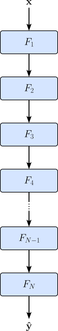
Each $F_i$ features a set of trainable parameters $\theta_i$ (e.g., weights and biases). If $\mathbf{h}_i$ denotes the output of $F_1$, we can define our network as:

$$\large \mathbf{h}_1 = F_1(\mathbf{h}_0;\theta_1),\quad \mathbf{h}_2 = F_2(\mathbf{h}_1;\theta_2), \dots, \quad \mathbf{h}_N = F_N(\mathbf{h}_{N-1};\theta_N), \quad \mathbf{\hat{y}} = \mathbf{h}_N $$

with loss some $\mathcal{L} = \mathcal{L}(\mathbf{y},\mathbf{\hat{y}})$. During training, we need to compute the gradients for the loss with respect to all trainable parameters $\theta_i$ via backpropagation. For example, to compute the gradient with respect to the parameters (\theta_1), we again apply the chain rule, but now we must account for how $\theta_1$ influences the loss through all subsequent layers:

$$\large \frac{\partial \mathcal{L}}{\partial \theta_1} = \frac{\partial \mathcal{L}}{\partial \mathbf{h}_N} \cdot \frac{\partial \mathbf{h}_N}{\partial \mathbf{h}_{N-1}} \cdot \frac{\partial \mathbf{h}_{N-1}}{\partial \mathbf{h}_{N-2}} \cdots \frac{\partial \mathbf{h}_2}{\partial \mathbf{h}_1} \cdot \frac{\partial \mathbf{h}_1}{\partial \theta_1} $$

The key observation is that $\theta_1$ affects the loss only through its effect on $\mathbf{h}_1$, but that effect must propagate through all subsequent layers. Vanishing or exploding gradients arise from how these Jacobians behave when multiplied repeatedly. This is why early-layer parameters in very deep networks are particularly sensitive to such pathological behavior.

Vanishing gradients are particularly problematic because they effectively prevent the earliest layers of a deep network from learning meaningful updates. During backpropagation, the gradients for early-layer parameters become extremely small as they are multiplied through many Jacobians. As a result, the parameter updates in those layers are close to zero, even when the model's predictions are clearly wrong. In practice, this means that learning becomes concentrated in the later layers, while earlier layers remain nearly unchanged from their initialization.

This is especially harmful because early layers are responsible for constructing the fundamental feature representations that all later layers depend on. If these representations do not improve, the entire network is limited in its ability to learn useful hierarchical structure. In extreme cases, training can appear to "stall", where loss decreases very slowly or not at all, giving the impression that the model has stopped learning. To reduce the risk of vanishing gradients, various strategies are commonly deployed, including:

Choice of activation functions: Replaces saturating functions such as Sigmoid or Tanh) with functions that maintain a constant gradient of 1 such as ReLU for positive inputs.
Smart weight initialization: Random but "controlled" weight initialization scales the initial weight variance based on the number of input and output neurons in a layer. This ensures that the initial weight Jacobians prevent the gradient variance from collapsing as it passes through deep layers.
Normalization layers: Methods such as Batch Normalization or Layer Normalization dynamically standardize the mean and variance of layer inputs throughout training. This keeps the inputs centered in the high-gradient, non-saturated operational zones of the activation functions.
Residual connections (i.e., structural shortcuts)...the topic of this notebook!

Residual Connection — Adding Shortcuts¶

Basic Idea¶

The basic idea behind residual connections (or skip connections) is to change what a neural network layer is asked to learn, while also introducing an alternative path for information to flow through the network. Instead of forcing a stack of layers to directly learn a complete input-to-output transformation, a residual block learns a residual function. Concretely, a residual block computes a mapping $H(\mathbf{x})$, by summing the output of $F(\mathbf{x})$ and the input $\mathbf{x}$; i.e.:

$$\large H(\mathbf{x}) = F(\mathbf{x}) + \mathbf{x} $$

In line with our previous illustration, we can graphically represent this idea as shown below — in fact, the figure below shows why the name residual or skip connection.

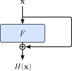
This skip connection creates a direct, alternative route through the network alongside the standard sequence of transformations. As a result, information can bypass intermediate layers when needed, while still allowing those layers to refine the representation. This makes deep networks significantly easier to optimize: if the optimal behavior is close to identity, the network can simply learn $F(\mathbf{x}) \approx 0$, effectively passing the input through unchanged.

Residual connections are typically not used for individual layers, but rather for groups of layers (residual blocks). The main reason is that a single layer transformation is usually too "small" and too tightly coupled with nonlinearities and parameterization to benefit much from a skip connection on its own. Instead, it is more meaningful to let a sequence of layers learn a richer transformation $F(\mathbf{x})$, and then add the input back at the end of that block. The figure below extends the previous example by showing the layers within $F_i$. In this simple example, we assume that the subnetwork consists of two linear layers and a nonlinear activation function.

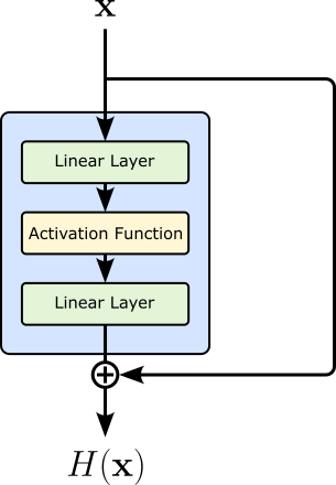
Notice that the last linear layer is also followed by a nonlinear activation function, but this activation function is typically applied after adding the residual connection. The motivation is that the residual branch and the identity shortcut should first be combined into a single representation before applying the nonlinearity. This preserves the idea that the block learns a correction to the identity mapping. Thus, more specifically and assuming some nonlinear activation function $\sigma$, the mapping $H(\mathbf{x})$ is defined as:

$$\large H(\mathbf{x}) = \sigma(F(\mathbf{x}) + \mathbf{x}) $$

Lastly, note that the basic definition $H(\mathbf{x}) = F(\mathbf{x}) + \mathbf{x}$ assumes that $F(\mathbf{x})$ and $\mathbf{x}$ matching shapes, otherwise we could not add them together. As a result, residual blocks are typically constructed in a way that preserves the dimensionality of the representation, allowing the identity shortcut to pass information through unchanged. However, this is not a strict requirement. When the input and output shapes differ the residual connection must be modified to make the addition valid. In these cases, the input is first transformed using a learnable mapping, often a linear layer or a $1 \times 1$ convolution, to align its shape with the output of the residual branch. This ensures that the core idea of residual learning is preserved even when the network changes representation size.

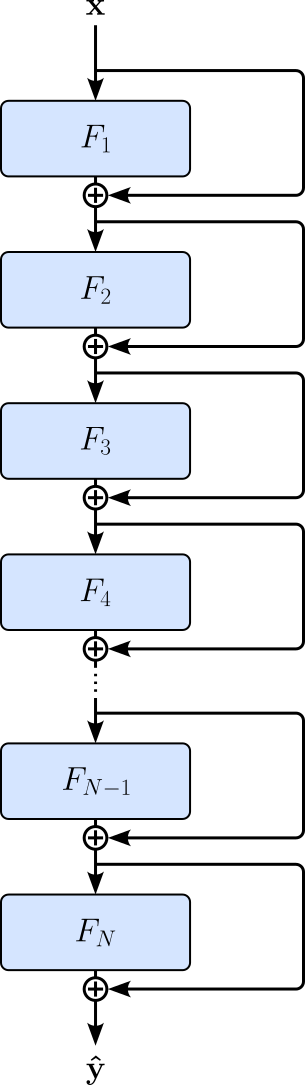
Most architectures using residual connections do not only have a single residual connection / residual block but multiple ones in the network's many layers. The figure below illustrates this idea by adding a residual connection to each module $F_i$ — here, we now assume that each $F_i$ is indeed a module with several layers instead of a single, say, linear layer.

Effects on Training¶

We saw that in network architectures without residual connections, gradients must pass through many consecutive Jacobian multiplications, which can cause gradients to shrink dramatically in very deep networks. Residual connections help train deep neural networks by introducing shortcut paths that allow information to flow through the network more directly. Instead of forcing all data to pass sequentially through every layer, skip connections create alternative routes that bypass one or more transformation layers. This means that if certain layers are not yet useful during training, the network can still preserve and propagate important information through the identity shortcut.

To better illustrate this, consider the following simple network containing $3$ residual connection / residual blocks.

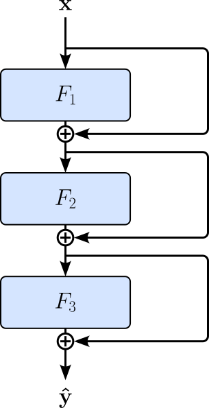
Similar to before, if we assume that $\mathbf{h}_i = F_i(\mathbf{h}_{i-1}) + \mathbf{h}_{i-1}$, as well as $\mathbf{h}_0 = \mathbf{x}$ and $\mathbf{h}_3 = \mathbf{\hat{y}}$, the outputs of the $3$ residual blocks are defined as follows — not that to omit the activation function applied to each some to ease presentation, and this details not important here:

$$ \begin{align} \large \mathbf{\hat{y}}\ &\large = F_3(\mathbf{h}_2) + \mathbf{h}_2\\[0.75em] \large \mathbf{h}_2\ &\large = F_2(\mathbf{h}_1) + \mathbf{h}_1\\[0.75em] \large \mathbf{h}_1\ &\large = F_1(\mathbf{x}) + \mathbf{x} \end{align} $$

Let's not express the output $\mathbf{\hat{y}}$ only in in terms of input $\mathbf{x}$ by replacing all intermediate result $\mathbf{h}_i$ of the residual blocks with their corresponding expression, giving us:

$$ \begin{align} \large \mathbf{\hat{y}}\ &\large = F_3(\mathbf{h}_2) + \mathbf{h}_2\\[0.75em] &\large = F_3(F_2(\mathbf{h}_1) + \mathbf{h}_1) + F_2(\mathbf{h}_1) + \mathbf{h}_1\\[0.75em] &\large = F_3(F_2(F_1(\mathbf{x}) + \mathbf{x}) + F_1(\mathbf{x}) + \mathbf{x}) + F_2(F_1(\mathbf{x}) + \mathbf{x}) + F_1(\mathbf{x}) + \mathbf{x}\\[0.75em] \end{align} $$

We can visualize this expression by an "unraveled view" of the network which shows all the possible paths from input $\mathbf{x}$ to output $\mathbf{\hat{y}}$. Each path is a unique configuration of which residual block to enter and which to skip.

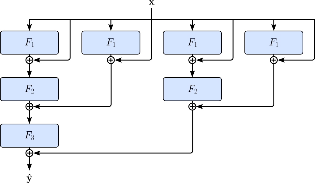
Since we have $3$ residual blocks, and each block gives us $2$ choices (enter or skip the block), there are $2^3=8$ unique paths the data can flow. In general, we have $k$ residual blocks, the number of unique paths is $2^k$. Residual connections provide a more direct path for gradients to flow backward through the network, helping preserve gradient magnitude and reducing the risk of vanishing gradients. In this sense, residual networks can be viewed as collections of many interconnected paths of different effective depths, making optimization significantly more stable and enabling the successful training of very deep neural networks.

Backward Pass¶

To actually see how residual connections behave during training, we need to look at how the computation of the gradients is done as part of the backward pass. Again, we assume the following basic implementation of a residual connection:

$$\large H(\mathbf{x}) = F(\mathbf{x}) + \mathbf{x} $$

When computing gradients during backpropagation, we apply the chain rule to both paths. The derivative of the output with respect to the input becomes:

$$\large \frac{\partial H(\mathbf{x})}{\partial \mathbf{x}} = \frac{\partial F(\mathbf{x})}{\partial \mathbf{x}} + \mathbf{I} $$

where $\mathbf{I}$ is the identity matrix (or simply $1$ in the scalar case). If we assume the residual block is part of some larger network — which is the most common situation in deep neural network architectures — during backpropagation, the block receives the upstream gradient $\large \frac{\partial \mathcal{L}}{\partial H(\mathbf{x})}$ from the previous layer (with respect to the backward pass). Consequently, the gradient of the loss $\mathcal{L}$ with respect to the input $\mathbf{x}$ is:

$$ \begin{align} \large \frac{\partial \mathcal{L}}{\partial \mathbf{x}}\ &\large= \frac{\partial \mathcal{L}}{\partial H(\mathbf{x})}\left(\frac{\partial F(\mathbf{x})}{\partial \mathbf{x}} + \mathbf{I}\right)\\[0.75em] &\large= \frac{\partial \mathcal{L}}{\partial H(\mathbf{x})} \cdot \frac{\partial F(\mathbf{x})}{\partial \mathbf{x}} + \frac{\partial \mathcal{L}}{\partial H(\mathbf{x})} \end{align} $$

This expression clear shows that, even if the gradient through the residual branch $\large \frac{\partial F(\mathbf{x})}{\partial \mathbf{x}}$ becomes very small, the residual connection still provides a direct path for gradients to flow backward. This is one of the main reasons residual connections help mitigate vanishing gradients and make very deep networks easier to train.

Basic Implementation¶

To show how we can implement a residual block, let's consider the simple example we shown before where the block consists of two linear layers and two activation functions — the second activation is not explicitly shown in the figure below but applied after summing up both branches.

The class ResidualBlock the code cell shows a conceptual implementation of this example; it assumes that we have class implementations of a linear layer and an activation function (here: ReLU). In the constructor, we define all required layers. Again, the last activation function self.relu2 is not explicitly shown in the previous figure.

forward(): This method takes in input $\mathbf{x}$ and passes it through the module containing the two linear layers with the first activation function between them. The output of this module is then added with input $\mathbf{x}$ — this forms the actual residual connection. Lastly, this combined output is then passed through the second linear layer to get the final output of the residual block.
backward(): This method essentially implements the expression for the backward pass we have seen above. The input argument of this method is the upstream gradient the residual block receives from the previous layer (previous with respect the the backward pass). The method then applies the chain rule to first compute the gradient with respect the second activation function relu2 — the output d represents $\large\frac{\partial \mathcal{L}}{\partial H(\mathbf{x})}$ in the expression above. Gradient d is then passed as the upstream gradient throught the module of the residual block: linear2 -> relu1 -> linear1. The resulting gradient dR represents $\large\frac{\partial \mathcal{L}}{\partial H(\mathbf{x})} \cdot \frac{\partial F(\mathbf{x})}{\partial \mathbf{x}}$. Then we only have to sum up both gradients d and dR to get $\large\large \frac{\partial \mathcal{L}}{\partial \mathbf{x}}$.

In [1]:

class ResidualBlock:
    
    def __init__(self, n_features):
        # Define layers of residual bloxk
        self.linear1 = Linear(n_features, n_features)
        self.relu1 = ReLU()
        self.linear2 = Linear(n_features, n_features)
        self.relu2 = ReLU()

    def forward(self, x):
        # Pass input through all layers in block
        out = self.linear1.forward(x)
        out = self.relu1.forward(out)
        out = self.linear2.forward(out)
        # Combine layer output with intial input
        out = out + x
        # Pass combined output through final activation function
        return self.relu2.forward(out)

    def backward(self, dY):
        # Gradient through final ReLU
        d = self.relu2.backward(dY)
        # residual branch backward
        dR = self.linear2.backward(d)
        dR = self.relu1.backward(dR)
        dR = self.linear1.backward(dR)
        # Combine gradients from skip and residual paths
        return dR + d

Again, this simple residual block assumes that the input and output have exactly the same shape — notice that both linear layers have the same input and output size of n_features — and that the residual connection is a pure identity mapping. If the shapes differ, the residual path must be modified using some projection layer to match dimensions before addition. The class would also need to be extended if more advanced residual designs are used. For instance, modern architectures like those in Deep Residual Learning for Image Recognition often include batch normalization layers, and some variants (pre-activation ResNets) change the ordering of normalization, activation, and convolution layers. In more complex systems, the residual branch itself may include multiple sub-blocks, dropout, or attention mechanisms.

Important: In modern deep learning frameworks such as PyTorch, a dedicated ResidualBlock class is often unnecessary because tensors are not just raw numerical arrays but objects that carry both data and an entire computation graph. When operations are applied to these tensor objects, the framework automatically records how each output depends on its inputs. This means that the forward pass alone is sufficient to define the full computation, and the backward pass can be derived automatically.

A key reason residual connections become so simple in these frameworks is operator overloading, especially for the + operator. When writing something like $H(\mathbf{x}) = F(\mathbf{x}) + \mathbf{x}$, the framework interprets this as an addition node in the computation graph and automatically constructs the correct gradient flow for both branches. During backpropagation, gradients are automatically split and routed through the residual path and the skip connection without any manual implementation. As a result, residual connections in PyTorch are typically implemented as a few lines of code inside a forward method, rather than requiring a custom backward implementation.

Discussion¶

Residual connections are a simple yet highly effective idea for improving the training of deep neural networks. Despite their simplicity, residual connections provide significant advantages when training very deep networks. They help mitigate problems such as vanishing gradients, allowing information and gradients to flow more easily through the network during backpropagation. As a result, deeper models become easier to optimize, converge faster, and often achieve higher accuracy. The success of residual connections, particularly in architectures such as ResNets, has demonstrated that even small architectural modifications can lead to major improvements in deep learning performance.

While residual connections can effectively mitigate the vanishing gradient problem and allowing networks to scale to thousands of layers, they do introduce several structural, mathematical, computational, and architectural constraints that may cause issues in practice:

Weaker "deep compositionality": We illustrated that residual networks may behave less like a single extremely deep model and more like an ensemble of many shallower subnetworks, because residual connections provide shortcut paths around blocks. Studies suggest that, during training, the network often relies most heavily on the shorter and easier optimization paths created by the identity shortcuts. As a result, during backpropagation, gradients tend to flow predominantly through these short paths rather than through long chains of nonlinear transformations. While this greatly improves optimization stability and helps avoid vanishing gradients, it may also reduce the degree to which very deep layers become strongly interdependent. In other words, some layers can effectively be bypassed without dramatically affecting network performance. As a result, residual networks may exhibit weaker "deep compositionality" than a purely sequential deep architecture, where each layer depends heavily on all preceding transformations. This tradeoff is part of what makes residual connections both highly effective for optimization and structurally different from traditional deep feedforward networks.
Computational overhead: Although residual connections appear computationally inexpensive because they only use simple element-wise additions $F(\mathbf{x}) + \mathbf{x}$, they can still introduce significant runtime overheads. During training, $\mathbf{x}$ must remain stored in memory until the computation of $F(\mathbf{x)$ is completed, increasing memory consumption substantially. In deep architectures, these shortcut connections can account for a large portion of the total feature map memory usage. Residual connections can also reduce hardware efficiency. Element-wise addition operations require considerable memory bandwidth despite involving relatively little computation, which can limit the performance of GPUs and TPUs that are optimized for highly parallel and contiguous operations. As a result, residual networks may experience slower inference speeds compared to simpler sequential architectures.
Risk of structural overfitting: Because residual connections open up a massive number of paths for information to travel through — see the example with $2^3=8$ paths in the example above — the functional capacity of the network scales drastically. If the training dataset lacks sufficient complexity or volume, deep networks with many residual connections are highly prone to structural overfitting. This often requires additional regularization techniques such as Stochastic Depth (randomly dropping residual blocks during training) or aggressive data augmentation just to keep the model from memorizing the noise in the training set.
Rigidity in model pruning and architecture search: Residual connections based on element-wise addition typically require the input $\mathbf{x}$ and the residual branch output $F(\mathbf{x})$ to have matching shapes. While this makes skip connections simple and efficient, it also introduces architectural rigidity. This may become problematic in case of model pruning and architecture optimization. Pruning inside one residual block changes its output dimensions, which can create incompatibilities with the identity shortcut. As a result, pruning decisions cannot easily be made independently for individual layers. Attempts to avoid this by pruning only internal hidden layers can lead to "hourglass"-shaped blocks, where narrow bottleneck layers reduce the representational capacity of the network and may hurt performance.

Despite these limitations and tradeoffs, residual connections have become standard components of modern deep learning architectures because their practical benefits overwhelmingly outweigh their drawbacks. By substantially improving optimization stability and enabling the successful training of very deep neural networks, residual connections have played a central role in the development of high-performing models across computer vision, natural language processing, speech recognition, and many other domains.

Summary¶

Residual connections (or skip connections) are a simple but powerful architectural idea in deep learning. Instead of forcing a stack of layers to directly learn a full transformation $H(\mathbf{x})$, a residual block learns a correction $F(\mathbf{x})$ to the input and outputs $F(\mathbf{x}) + \mathbf{x}$. This introduces an alternative path through the network that allows information to flow more directly from earlier to later layers. As a result, deep networks can preserve useful information even when intermediate transformations are still being learned.

From an optimization perspective, residual connections significantly improve the training of deep neural networks. They help mitigate issues such as vanishing gradients by providing a direct route for gradient flow during backpropagation. Instead of gradients being repeatedly multiplied through many nonlinear transformations, part of the gradient can flow unchanged through the skip connection. This makes it easier to train very deep architectures and allows networks to scale to hundreds or even thousands of layers in practice.

We also explored a basic implementation of a residual block, consisting of a small subnetwork (e.g., linear layers with nonlinear activations) combined with an identity residual connection. The forward pass computes the residual branch and adds the original input, while the backward pass splits gradients into two paths: one through the residual branch and one through the identity shortcut. This illustrates how residual learning naturally decomposes both computation and gradient flow into parallel pathways.

Today, residual connections have become a standard building block in modern deep learning architectures, including convolutional networks, transformers, and diffusion models. Their simplicity, combined with their strong impact on optimization and scalability, makes them one of the most important architectural innovations in deep learning. Understanding residual connections is therefore essential for anyone working with or studying modern neural network systems.

In [ ]: