Disclaimer: This Jupyter Notebook contains content generated with the assistance of AI. While every effort has been made to review and validate the outputs, users should independently verify critical information before relying on it. The SELENE notebook repository is constantly evolving. We recommend downloading or pulling the latest version of this notebook from Github.
Recurrent Neural Networks — An Introduction
Recurrent Neural Networks (RNNs) are a class of artificial neural networks designed for sequential data processing. Unlike traditional feedforward neural networks, RNNs have connections that allow information to persist, making them well-suited for tasks where previous inputs influence future outputs. This unique structure enables RNNs to recognize patterns in time-series data, natural language, and other sequences, making them essential for applications like speech recognition, language modeling, and financial forecasting.
What makes RNNs special is their ability to maintain a form of memory through hidden states, allowing them to process sequential information efficiently. Standard neural networks process inputs independently, while RNNs consider past inputs through their recurrent connections. This characteristic makes them powerful for applications requiring context awareness, such as machine translation, where understanding previous words is crucial to predicting the next. However, traditional RNNs suffer from limitations like vanishing gradients, which make it difficult for them to remember long-term dependencies. To address these challenges, advanced architectures like Long Short-Term Memory (LSTM) and Gated Recurrent Units (GRU) have been developed.
Learning about RNNs is important because they are foundational to many modern AI advancements. Many real-world applications, including chatbots, predictive text, and automated translation services, rely on RNNs or their improved variants. Understanding how RNNs work helps in developing more efficient and intelligent systems for processing sequential data. Additionally, knowledge of RNNs provides insight into how AI models can be optimized for better performance, ensuring that they function effectively in complex real-world scenarios.
Furthermore, mastering RNNs opens doors to research and innovation in artificial intelligence. With the rise of deep learning and natural language processing, many cutting-edge technologies, such as transformers and generative AI models, have evolved from RNN-based concepts. By studying RNNs, one can appreciate the evolution of AI models and gain the necessary skills to contribute to future developments in machine learning. Thus, RNNs serve as a crucial stepping stone for anyone interested in advancing their expertise in artificial intelligence.
Setting up the Notebook
Make Required Imports
This notebook requires the import of different Python packages but also additional Python modules that are part of the repository. If a package is missing, use your preferred package manager (e.g., conda or pip) to install it. If the code cell below runs with any errors, all required packages and modules have successfully been imported.
import torch
import torch.nn as nn
What is Sequential Data
Sequential data is data where the order of elements matters because it contains an inherent structure over time or position. Each data point depends on the previous ones, making sequence relationships crucial for analysis. Common examples for sequential data include:
Time Series Data: Time-series data consists of observations recorded at successive time intervals, making the order of data points crucial for analysis. Common examples include financial data, such as stock prices, exchange rates, and cryptocurrency values, where past trends influence future predictions. Weather data, like temperature, humidity, and precipitation levels over time, is another example where sequential dependencies help forecast future conditions. In healthcare, patient monitoring data, such as heart rate and blood pressure readings over time, must be treated sequentially to detect abnormalities and predict potential health risks. Other important examples include sensor data from IoT devices, such as electricity usage in smart grids or vibration data from industrial machines, where analyzing past patterns helps predict failures or optimize performance. In transportation, GPS tracking data from vehicles is used for traffic prediction and route optimization.
Natural Language Text: Natural language is considered sequential data because the meaning of words and sentences depends on their order. In a sentence, words appear in a structured sequence, where changing the order can alter or completely distort the intended meaning. For example, "The cat chased the mouse" has a different meaning than "The mouse chased the cat." This sequential dependency makes language processing tasks, such as machine translation, speech recognition, and text generation, highly reliant on models that can understand word relationships over time. Additionally, linguistic structures like grammar, syntax, and context require maintaining a memory of previous words to correctly interpret the next ones. For instance, in a long sentence or paragraph, understanding a pronoun like "it" depends on recognizing the noun it refers to earlier in the text.
Speech and Audio Data: Speech and audio data are considered sequential because they consist of continuous signals that evolve over time, where the order of sound waves or digital samples is essential for understanding meaning. In speech, phonemes (the smallest units of sound) must follow a structured sequence to form words and sentences. If the order is altered, the meaning of spoken language can change entirely or become unintelligible. For example, in speech recognition, the phrase "open the door" must be processed in the correct sequence to distinguish it from a similar-sounding but different phrase like "the door open". Beyond speech, other forms of audio data, such as music or environmental sounds, also rely on sequential relationships. In music, for instance, notes and rhythms must follow a specific order to create a melody, and a disruption in this sequence alters the musical structure. Similarly, in sound classification tasks, the progression of audio events—such as footsteps followed by a door creaking—provides context for interpretation. Audio models often use spectrogram representations, where time is one axis and frequency is another, preserving the sequential nature of sound. Because understanding speech and audio depends on recognizing patterns over time, treating them as sequential data is crucial for accurate processing in AI applications.
Video Data: Video data is considered sequential because it consists of a series of frames displayed in a specific order over time, where each frame is dependent on the ones before and after it. Unlike static images, which can be analyzed independently, videos capture motion, making temporal relationships crucial for understanding actions, events, and transitions. For example, in action recognition, distinguishing between a person standing up and sitting down requires analyzing how their position changes across multiple frames. If the frames were shuffled or analyzed separately, the sequence of movement would be lost, leading to incorrect interpretations. Moreover, many video-based AI applications, such as object tracking, gesture recognition, and video captioning, rely on understanding changes in the scene over time. In self-driving cars, for instance, video from cameras is used to track moving objects like pedestrians and other vehicles, where sequential processing helps predict future positions.
Biological Sequences: Biological sequences, such as DNA, RNA, and protein sequences, are considered sequential data because their structure and function depend on the specific order of their components. In DNA and RNA, nucleotides (A, T, C, G for DNA; A, U, C, G for RNA) are arranged in a precise sequence that encodes genetic information. Any change in this order, such as a mutation, can alter gene expression and potentially lead to biological changes or diseases. Since the meaning of a sequence depends on the position and arrangement of nucleotides, analyzing them as sequential data is essential for tasks like gene prediction, mutation detection, and evolutionary analysis. Similarly, protein sequences consist of amino acids arranged in a linear chain, where the sequence determines the protein's structure and function. Protein folding, interactions, and biological activity all depend on the correct ordering of amino acids.
Event Sequences: Event sequences are ordered lists of events that occur over time, where the sequence of occurrences holds meaningful patterns and dependencies. These events can represent various real-world activities, such as user interactions on a website, medical records of patient visits, or system logs in cybersecurity. The order in which events happen is crucial for understanding behavior, predicting future actions, and detecting anomalies. For example, in customer behavior analysis, tracking the sequence of clicks, purchases, and cart abandonments helps businesses personalize recommendations and improve user experience. Event sequences are considered sequential data because their meaning and interpretation depend on temporal ordering. Changing the order of events can alter their significance or lead to incorrect predictions. In fraud detection, for instance, a sudden sequence of high-value transactions followed by an account login from a different country might indicate fraudulent activity.
To capture the sequential nature of the data, we need to use a suitable representation to describe a data sample $\mathbf{x}$. The most common and straightforward way is describe a sample of sequential data as a list of the sequence elements:
Here we assume that each element is a feature vector — for example, the feature vector for time series data, word embedding vectors in case of text, image frames in case of video data, and so on (of course, each $\mathbf{x}_t$ can be a vector with a single element so that the each feature vector collapses to a scalar feature values). Note that in practice, this sequence of vectors is typically implemented as a matrix (or a tensor in case of additional dimensions). In this representation, $T$ marks the length of the sequence, and $\mathbf{x}_t$ marks the feature vector at time stamp $t$ — the notion of a time step is commonly used even for non-time series data such as words in a text or frame in a video.
Throughout this notebook, we will consider natural language text as example data to motivate and introduce Recurrent Neural Networks. RNNs gained widespread popularity in machine learning precisely because of their success in processing natural language data. Common tasks where RNNs are used include text generation, sentiment analysis, and machine translation. Before the rise of Transformer-based models, RNNs and their variants, such as Long Short-Term Memory (LSTM) networks and Gated Recurrent Units (GRUs), were the backbone of many state-of-the-art language models. By using text as an example, we can illustrate how RNNs handle sequential dependencies, predict the next word in a sentence, and generate meaningful text based on prior inputs. In short, in the following, $\mathbf{x}$ denotes a single sentence, and $\mathbf{x}_t$ is a word embedding vector (e.g., a pretrained embedding vectors based on Word2Vec, GloVe, FastText, etc.).
From FFNs to RNNs
A good way to understand the basic idea behind Recurrent Neural Networks is first understand the limitations of Feed-Forward Neural Networks and what RNNs add to the FFN architecture to address these limitations. So let's do this in this section step by step.
Quick Refresher: FFNs
Feed-Forward Neural Networks (FNNs) are one of the most fundamental types of artificial neural networks, designed for mapping input data to output predictions. They consist of an input layer, one or more hidden layers, and an output layer, where information flows in one direction — from input to output — without any cycles or loops. Each neuron in a layer is connected to neurons in the next layer, and these connections have weights that adjust during training to optimize performance. The network learns patterns from data using activation functions and backpropagation, a process that updates weights based on error minimization. FNNs are widely used for tasks such as image recognition, classification, and regression due to their simplicity and effectiveness. They serve as the foundation for more advanced deep learning models and are especially useful when working with structured, non-sequential data.
A Simple FFN Example
To given an example, the image below shows the architecture of a very simply FNN consisting of
- an input layer with 3 features
- a single hidden layer with 4 neurons, and
- an output layer with to neuron (e.g., for a binary classification task)
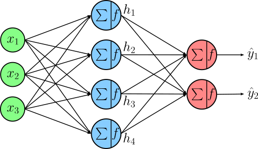
Again, just from looking at the architecture image, appreciate that the information flows in one direction from the input to the output — that is, the inputs are used to calculate the output of the hidden layer, and these results are used to calculate the final output of the output layer. If $\mathbf{x} = (x_1, x_2, x_3)^T$ denotes the input vector, $\mathbf{h} = (h_1, h_2, h_3, h_4)^T$ denotes the output vector of the hidden layer, and $\mathbf{\hat{y}} = (\hat{y}_1, \hat{y}_2)^T$ denotes the output vector of the output layer, we can express the calculations done by the example FNNs using the following equations.
Where $\mathbf{W}_{xh}$ and $\mathbf{W}_{hy}$ are the weight matrices of the hidden layer and the output layer, respectively; $\mathbf{b}_{h}$ and $\mathbf{b}_{y}$ are the corresponding biases. Functions $f_h$ and $f_y$ are suitable activation functions. For example, assuming a binary classification task the function of choice for $f_y$ is the Softmax function to ensure that the outputs can be interpreted as probabilities. Since $f_h$ is the activation of this hidden layer, we have more choices for its exact implementation. Common choices include ReLU, Tanh, Sigmoid, and others.
Limitations of FFNs
In principle, Feed-Forward Neural Networks (FNNs) can be effectively used for text classification (e.g., spam detection, sentiment analysis, and topic classification) by transforming textual data into numerical representations, such as Term Frequency-Inverse Document Frequency (TF-IDF) vectors based on the Vector Space Model. Here, the TF-IDF vector representing a document forms the input vector $\mathbf{x}$. However, document vectors based on the Vector Space Model (with TF-IDF or alternative weights) have several limitations:
Loss of word order and context. TF-IDF treats each word as an independent feature, disregarding the order in which words appear. This means that two sentences with the same words but different structures (e.g., "The cat chased the dog" vs. "The dog chased the cat") will have identical TF-IDF representations. Since FNNs process these vectors without considering word order, they fail to understand contextual meaning.
Lack of semantic understanding. TF-IDF assigns importance based purely on word frequency, without capturing the actual meaning of words. For example, synonyms like "happy" and "joyful" will have different vector representations even though they convey the same sentiment. This limitation prevents FNNs from generalizing well in text classification tasks that require semantic understanding. In contrast, word embeddings (e.g., Word2Vec, GloVe) to represent individual words and not whole documents provide more meaningful representations by considering word relationships.
Sparse and high-dimensional features. Since TF-IDF vectors are typically very large (with one dimension per word in the vocabulary), they create sparse representations, where most values are zero. This sparsity can make learning inefficient in FNNs, as neural networks perform better with dense and meaningful representations. High-dimensional inputs also increase computational complexity and the risk of overfitting, especially when training on limited data.
Difficulty in capturing long-term dependencies. TF-IDF does not retain any information about long-range dependencies between words. For instance, in sentiment analysis, words expressing sentiment ("not bad" vs. "very bad") may be far apart in a sentence, but TF-IDF treats them as independent features. Since FNNs process inputs in a static way, they cannot capture these dependencies. While including bigrams, trigrams, etc. address word dependencies to some extent, they also increase the total number of features.
In short, using FFNs to train, say, a text classification model using TF-IDF document vectors is typically only meaningful if the predictions are very likely depend on the presence and absence of words (or more generally: n-grams) alone. However, text is first and foremost sequential data, and many important semantics are captured by the word order and (long-term) dependencies between words in a document. FFNs are generally not capable of capturing these types of information underlying a phrase, sentence, paragraph, or document. Of course, assuming sequential data of the form:
we could give each word embedding vector to $\mathbf{x}_t$ to and FFN one by one during training. However, the FFN would not be able to capture any relationships between the words of the input sentence. We therefore need some way for the network to "remember" some previous result from inputs $\mathbf{x}_1, \mathbf{x}_2, \dots, \mathbf{x}_{t-1}$ when processing $\mathbf{x}_t$. This brings us to the idea of the hidden state and recurrence.
The Heart of RNNs: The Hidden State & Recurrence
To better understand the core idea of RNNs, let's have a last look at our initial example FFN architecture. The image below shows an abstraction of the FNN by combining all inputs and neurons of the same layer into a single node. In other words, each node in the image below represents a complete layer containing all the inputs and neurons of that layer.
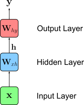
Of course, this simplified representation does not change the models behavior: it takes a single vector $\mathbf{x}$ is input (e.g., a TF-IDF document vector), uses $\mathbf{x}$ to calculate the output $\mathbf{h}$ of the hidden layer, and finally uses $\mathbf{h}$ to calculate the single output vector $\mathbf{y}$. Based on this representation, we will see in a moment how RNNs support the processing of sequential data such as text.
As mentioned before, we could replace a single document vector $\mathbf{x}$ with a sequence of word embedding vectors $\mathbf{x} = [\mathbf{x}_1, \mathbf{x}_2, \mathbf{x}_3, \dots ]$ and give the FFN each word embedding vector $\mathbf{x}_t$ as input and use all $T$ outputs to somehow make a final prediction. Still, we would not be able to capture any relationship between the words using this approach.
To accomplish this, RNNs introduce the concept of a hidden state. The hidden state is an additional vector incorporated into the network that commonly holds the output $\mathbf{h}$ of the hidden layer — although the hidden state can be arbitrarily further manipulated. As such, the size of the hidden state is typically simply the size of the hidden layer. With this hidden state the RNNs retains information from previous time steps, allowing the model to capture dependencies in sequential data. Mathematically, the hidden state at time step $t$ can be expressed using the following recurrent formula:
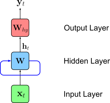
In other words, the hidden state $\mathbf{h}_t$ at time step $t$ is some function of the hidden state $\mathbf{h}_{t-1}$ from previous timestamp $(t-1)$ and of the input feature vector $\mathbf{x}_t$ (e.g., a word embedding vector) at time step $t$. There are different common ways to actually implement the function $f_{\mathbf{W}}$ which yield different RNN variants; as we will see later. We can visualize this recurrent formula using out abstract representation of a neural network by adding adding a loop (blue edge) reflecting that the inputs of the hidden layers are now both the current input $\mathbf{x}_t$ and the previous output of the hidden layer retained by the hidden state.
When looking at the recurrent formula for $\mathbf{h}_t$, the natural questions about $\mathbf{h}_0$ arises. After all, even for the first input vector $\mathbf{x}_1$ to calculate $\mathbf{h}_1$ the formula expects $\mathbf{h}_0$ as input. Initializing the hidden state of a Recurrent Neural Network (RNN) is crucial for ensuring stable training and good model performance. There are several common approaches to initializing the hidden state:
Zero Initialization: The most common and straightforward approach is to initialize the hidden state as a vector of zeros. This ensures consistency and does not introduce any bias at the beginning of training. While this is often sufficient, it may slow down convergence in some cases, especially for deep RNNs with many layers.
Random Initialization: Instead of using zeros, the hidden state can be initialized with small random values, typically sampled from a normal or uniform distribution. This can help break symmetry and encourage diverse learning patterns. However, improper scaling of random initialization may lead to instability in training.
Learnable Parameters: Some architectures treat the initial hidden state as a set of trainable parameters that are learned during training. This allows the network to optimize the starting point for each sequence and can improve performance, particularly in tasks where the initial state carries meaningful information.
Using a Separate Network or Prior Knowledge: In some advanced applications, such as language modeling or reinforcement learning, the initial hidden state can be derived from another network, pre-trained embeddings, or external knowledge about the data. For example, in sequence-to-sequence models, the encoder's final hidden state is often used to initialize the decoder's hidden state.
The choice of initialization depends on the specific task and model architecture. While zero initialization works well in many cases, learnable or task-specific initializations can lead to better performance in more complex settings. To better visualize the importance of initial hidden state $\mathbf{h}_0$ and the evolution of the hidden state across all time steps, we can "unroll" our network architecture, to show the network at each time step and which inputs the hidden layer receives at each time step.
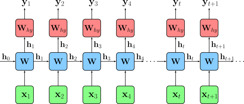
Again, note that hidden and output layer at each time step represent the same network.
Vanilla RNN Implementation
So far, we only considered the general form of the recurrent for $h_t = f_{\mathbf{W}}(\mathbf{h}_{t-1}, \mathbf{x}_t)$. We still need to define how to implement function $f_{\mathbf{W}}$. The simplest form of $f_{\mathbf{W}}$ that is commonly used in practice — therefore often also called Vanilla RNN — is implemented using the following function for $\mathbf{h}_t$ (function $f_y$ remains unchanged):
This means that the hidden layer now has 2 weight matrices $\mathbf{W}_{hh}$ and $\mathbf{W}_{xh}$ to first transform the previous hidden state $\mathbf{h}_{t-1}$ and the current input vector $\mathbf{x}_t$, respectively. These weight matrices (and the bias vector $\mathbf{b}_h$) contain all trainable parameters of the hidden layer. Apart from increasing the capacity for the model to learn complex relationships, having both weight matrices also makes it easy to ensure that the results of $\mathbf{W}_{hh}\mathbf{h}_{t-1}$ and $\mathbf{W}_{xh}\mathbf{x}_{t}$ have the same size and can therefore be added — typically the size of the hidden states $\mathbf{h}_t$ is different from the size of the input vectors $\mathbf{x}_t$. This simple implementation of the recurrent formula is typically depicted using the following abstract visualization.
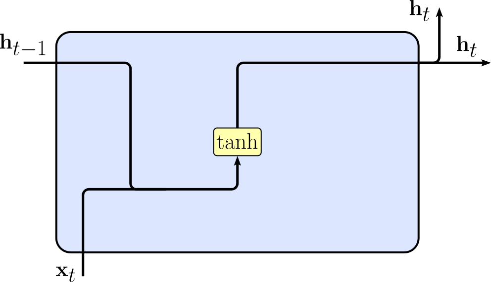
While this visualization may not look very exciting, it will later helps to better appreciate the more complex implementations of the recurrent formula, which will bring to the more sophisticated RRN variants Long Short-Term Memory (LSTM) networks and Gated Recurrent Units (GRUs).
Side note: this component of the network that implement the recurrent formula is often called the cell; for example, the basic implementation above would be called the Vanilla RNN cell. Conceptually, the cell is just the modified/extended hidden layer. However, since this step involves not more than a simple linear transformation — particularly in the case of LSTMs and GRUs — the term cell is commonly used to distinguish it from a normal hidden layer and to emphasize the connections to RNNs.
To make this idea of a Recurrent Neural Network more tangible, let's actually implement a toy RNN using PyTorch. For this, the code below shows the implementation of the Vanilla RNN cell. Of course, using input arguments for the constructor, we need to tell the network module the size of the input vector and the size of the hidden state — again, they do not have to have the same size. The module defines the two weight matrices $\mathbf{W}_{hh}$ and $\mathbf{W}_{xh}$ using standard nn.Linear layers. Notice that the output size of both linear layers is the size of the hidden state to ensure that after both transformations the sizes do match. The forward() method directly implements the basic recurrent formula for the current hidden state $\mathbf{h}_t$ and returns it.
class VanillaRNNCell(nn.Module):

    def __init__(self, input_size, hidden_size):
        super().__init__()
        self.Wxh = nn.Linear(input_size, hidden_size)
        self.Whh = nn.Linear(hidden_size, hidden_size)

    def forward(self, inputs, hidden):
        return torch.tanh(self.Wxh(inputs) + self.Whh(hidden))
Notice how this implementation slightly differs from the recurrent formula: Since we are using two nn.Linear layers, each of them comes with its own bias vector $\mathbf{b}$. This means that the cell has two bias vectors $\mathbf{b}_{xh}$ and $\mathbf{b}_{hh}$ instead of just a single bias vector $\mathbf{b}_{h}$ (cf. the definition of the recurrent formula above). However, this generally does not affect the overall capacity of the network. While the implementation could be changed to exactly match the recurrent formula, it removes some of the simplicity of the code.
Now let's actually define a Vanilla RNN cell that we can use. For this we assume word embedding vectors as input. A common size of pretrained word embedding vectors is $300$, so let's use this value as our input size. Similarly, a common size of the hidden state, i.e., the output of the hidden layer, is 512. Of course, you can change these values to see the effects. However, for the following discussion we assume the default values of 300 and 512 for the size of the word embedding vectors and the hidden state, respectively.
# Define the sizes of the input vectors and of the hidden state
input_size, hidden_size = 300, 512

# Define Vanilla RNN cell based on given vector sizes
vanilla_rnn_cell = VanillaRNNCell(input_size, hidden_size)

# Print cell (which is a PyTorch nn.Module)
print(vanilla_rnn_cell)
VanillaRNNCell(
  (Wxh): Linear(in_features=300, out_features=512, bias=True)
  (Whh): Linear(in_features=512, out_features=512, bias=True)
)
We can also "run" the RNN cell by giving it some random input and observing the output. To this end, in the code cell below, we first create some random batch of feature vectors. Using the the default values — of course, you can change those if you want — we create a batch of size 4 containing all first elements $\mathbf{x}_1$ in the 4 sequences; the size of the input vectors is taken from above (by default: 64). At the end, we only have a look at the shapes of the batch and the hidden state; since the batch and the hidden state were initialized randomly, looking at the actuals value is not really meaningful.
# Define size of input batch
batch_size = 64

# Create a random first input batch
x1 = torch.rand((batch_size, input_size))

#Initialize hidden state h0 using basic zero initialization
h0 = torch.zeros(batch_size, hidden_size)

print(f"Shape of input batch x1:  {x1.shape}")
print(f"Shape of hidden state h0: {h0.shape}")
Shape of input batch x1:  torch.Size([64, 300])
Shape of hidden state h0: torch.Size([64, 512])
With $\mathbf{x}_1$, $\mathbf{h}_0$, and the RNN cell defined, we can now calculate $\mathbf{h}_1$. The only difference compared to our conceptual introduction of the hidden state and the recurrent formula is that we now work with batches of sequences and not individual sequences — and we typically try to work with batches in practice for performance reasons. However, this is completely handled under the hood by PyTorch.
h1 = vanilla_rnn_cell(x1, h0)

print(f"Shape of output: {h1.shape}")
Shape of output: torch.Size([64, 512])
Unsurprisingly, each output vector of the RNN cell (i.e., the hidden layer) of size $512$ for each of our 64 input vectors.
The RNN cell is only a component of the network. Most importantly, we also need an output layer to generate the final output $\mathbf{y}_t$. But with our implementation of VanillaRNNCell, we can now implement the complete network model as the class VanillaRNN as shown in the code cell below. Apart from the Vanilla RNN cell, this class also defines the weight matrix $\mathbf{W}_{hy}$ to transform the hidden state to the output. Assuming this network implements some classification task, we can also include the Softmax function as the final layer. The forward() method calculates the current hidden state $\mathbf{h}_t$ and the final output $\mathbf{y}_t$ and returns them both.
class VanillaRNN(nn.Module):

    def __init__(self, input_size, hidden_size, output_size):
        super().__init__()
        self.cell = VanillaRNNCell(input_size, hidden_size)
        self.Why  = nn.Linear(hidden_size, output_size)
        self.out  = nn.Softmax(dim=1)

    def forward(self, inputs, hidden):
        hidden = self.cell(inputs, hidden)
        output = self.out(self.Why(hidden))
        return output, hidden
To create an example network, let's assume we consider classification tasks with $10$ class labels. This means that the number of neurons in the output layer will also be $10$. Together with the previous choice for the size of the input vectors and the size of the hidden layer, we have all required arguments to define out VanillaRNN model; see the the code cell below.
# Define size of the ouput (default: 10-class classification task)
output_size = 10

# Define complete Vanilla RNN Network
vanilla_rnn = VanillaRNN(input_size, hidden_size, output_size)

# Print cell (which is a PyTorch nn.Module)
print(vanilla_rnn)
VanillaRNN(
  (cell): VanillaRNNCell(
    (Wxh): Linear(in_features=300, out_features=512, bias=True)
    (Whh): Linear(in_features=512, out_features=512, bias=True)
  )
  (Why): Linear(in_features=512, out_features=10, bias=True)
  (out): Softmax(dim=1)
)
Finally, we can give our model a batch of sequences as input. Using the default value in the code cell below, we assume that all sequences in the example batch have a length of $20$. After creating our random input batch x we also need to initialize our first hidden state vector $\mathbf{h}_0$; again, here we do this just randomly. The loop then iterates through all sequences in the batch, fetches the $t$-th input vector from each sequence. Notice that the shape of the batch x is (batch_size, seq_len, hidden_size), indicating that the 2nd dimension of the batch is the sequence length dimension. When can give the current input vector $\mathbf{x}_t$ and the previous hidden state $\mathbf{f}_{t-1}$ to our VanillaRNN instance to get the output $\mathbf{y}_t$ and the new hidden state $\mathbf{h}_t$ — note that we just call the hidden state h since we simple overwrite it in each iterations.
# Specify length of all sequences in the batch
seq_len = 20

# Create a randon input batch of size batch_size with sequences of length sew_len
x = torch.rand((batch_size, seq_len, input_size))

#Initialize hidden state h0 using basic zero initialization
h = torch.zeros(batch_size, hidden_size)

for t in range(x.shape[1]):
    # Get input batch for time step t
    xt = x[:,t,:]
    # Calculate output based current input and previous hidden state (and overwrite hidden state for next iteration)
    yt, h = vanilla_rnn(xt, h)
    # ... do something meaningful with the output ...
Clearly, this code cell does nothing meaningful, let alone any training. The purpose of the example code was merely to illustrate the sequential processing of a batch of input sequences. If we would train this model, we would need to calculate the loss with respect to the predictions and some ground truth class labels based on some training dataset. But that already goes beyond this introductory notebook and will be covered in other notebooks. Of course, Neural Network libraries such as PyTorch, Tensorflow, and others provide configurable implementations of Recurrent Networks that handle this iterative process under the hood.
Common Sequence Task for RNNs
Recurrent Neural Networks are very versatile neural network architecture that can be used to solve a wide range of sequence-based tasks. In the following we briefly discuss the four basic types of sequence-based tasks and illustrate their basic implementation using RNNs. While the examples below focus on natural language data, the same ideas apply for other types of sequence data.
Many-to-One
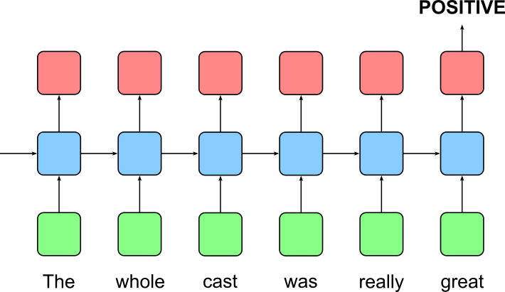
A many-to-one sequence task in machine learning refers to a problem where a model processes a sequence of inputs and produces a single output. A classic example of a many-to-one task is sentiment analysis, where an RNN processes an entire sentence or paragraph and predicts whether the sentiment is positive or negative (assuming a binary classification). Here the input, i.e., each word/token in a sentence, is processed step by step until the last word/token at time step $T$, and the hidden state gets updated along the way. Then, the last hidden state $\mathbf{h}_T$ is used as input for one or more additional layers to get the final output. The image below illustrates the idea using the unrolled representation of an RNN for a sentiment analysis use case.
One-to-Many
A one-to-many sequence task in machine learning involves a scenario where the model receives a single input and generates a sequence of outputs. This setup is particularly common in generative tasks, where the initial input serves as a seed or context, and the model must produce a series of related elements. For example, in image captioning, a model might take a single image as input and then generate a descriptive sentence word by word. Similarly, in music generation, a model might start with a specific motif or chord and then generate a sequence of notes that form a complete melody. By sequentially producing each element based on the initial input and the previously generated outputs, the model ensures that the final output sequence is contextually relevant and well-structured. This approach is widely used in natural language processing, creative content generation, and various other domains where producing an ordered sequence of outputs is essential.
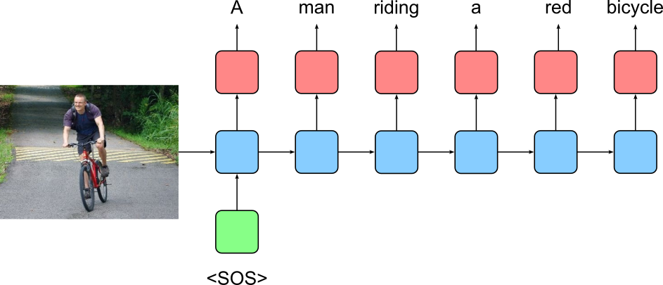
The image below shows the basic setup of using RNN for image captioning. Here, we assume that the image has been somehow encoded — typically using a Convolutional Neural Network or similar architecture to serve as the initial hidden state $\mathbf{h}_0$ of the RNN. A special word/token (here: "<SOS>") that serves as initial input for the RNN is used to kick-start the generation of the sequence of words/tokens to form the image caption.
Many-to-Many: Sequence Labeling
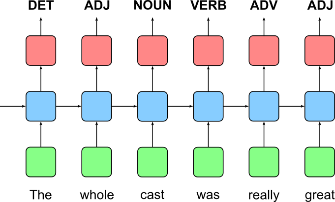
A many-to-many sequence task for labeling sequences in machine learning involves processing an input sequence and generating an output sequence typically the same length — although the length may differ for certain use cases — where each input element is assigned a corresponding label. This type of task is commonly used in applications where every time step in the input sequence requires a classification or annotation. For instance, in Named Entity Recognition (NER), each word in a sentence is labeled as a proper noun, location, organization, or other entity type. Similarly, in Part-of-Speech (POS) tagging, each word is classified as a noun (NOUN), verb (VERB), adjective (ADJ), adverb (ADV), determiner (DET), etc., making it a crucial component of natural language processing (NLP). The image below shows how an RNN can be used to solve a POS tagging task using a simple example sentence.
Many-to-Many: Encoder-Decoder Architecture
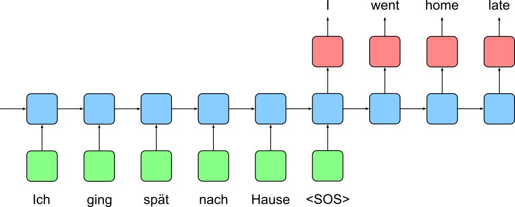
A many-to-many sequence task for text generation using an encoder-decoder architecture involves processing an input sequence and generating an output sequence, where both sequences may have different lengths. This approach is commonly used in tasks like machine translation, where an entire sentence in one language (e.g., German) is taken as input, encoded into a latent representation, and then decoded into a sentence in another language (e.g., German). The encoder compresses the input sequence into a context vector, capturing its meaning, while the decoder generates the output sequence step by step, maintaining coherence and structure. This encoder-decoder structure allows models to generate fluent, context-aware sequences, making it a cornerstone of modern natural language processing (NLP) tasks.
The image below illustrates encoder-decoder architecture using two Recurrent Neural Networks for a machine translation task (German to English). The encoder RNN reads in the input sentence in the source language (here: German) resulting in the last hidden state $\mathbf{h}^{enc}_T$ of the decoder. This hidden state is then used to initialize the hidden state for the decoder RNN, i.e., $\mathbf{h}^{dec}_o = \mathbf{h}^{enc}_T$. Again, we use some special word/token (here: "<SOS>") to start the generation of the text in the target language (here: English) by the decoder RNN.
The purpose of the previous examples was to illustrate on a fairly high level how RNNs can be used for different types of sequence-based tasks. Their different challenges and practical examples will be the subject of separate notebooks. The main take-away message here is the versatility of Recurrent Neural Networks for machine learning given sequential data.
RNN Variants & Extensions
RNN Variants
Recall that the basic concept of a Recurrent Neural Network is reflected in the recurrent formula
We also saw the most basic implementation of that formula that gives us the Vanilla RNN cell. Just as a reminder, the image below shows the visualization of the Vanilla RNN cell.
The main problem with the Vanilla RNN cell is the vanishing and exploding gradient problem, which makes training deep or long-sequence models difficult. Since RNNs update their hidden states at each time step using backpropagation through time (BPTT), gradients are repeatedly multiplied as they propagate backward through the network. If these gradients are small (less than 1), they shrink exponentially, causing the model to forget long-term dependencies — this is known as the vanishing gradient problem. Conversely, if gradients are large (greater than 1), they grow exponentially, leading to instability in training — this is called the exploding gradient problem.
Due to the vanishing gradient problem, Vanilla RNNs struggle to learn dependencies over long sequences, as older time steps have little to no influence on the final output. This limits their ability to model tasks requiring long-range context, such as language translation or speech recognition. The exploding gradient problem, on the other hand, causes large weight updates that make training unstable, though it can be controlled using gradient clipping. To address these limitations, advanced RNN architectures like Long Short-Term Memory (LSTM) and Gated Recurrent Unit (GRU) were introduced, as they use gating mechanisms to better retain and manage long-term dependencies. Let's have a brief and high-level look at LSTMs and GRUs to appreciate their added complexity and their differences.
Long Short-Term Memory (LSTM)
Long Short-Term Memory (LSTM) networks were first proposed in 1997 by Sepp Hochreiter and Jürgen Schmidhuber in their paper titled "Long Short-Term Memory". The key difference between a Vanilla RNN cell and an LSTM cell lies in how they handle long-term dependencies in sequential data. A Vanilla RNN cell is the simplest form of a recurrent unit that maintains a single hidden state, which gets updated at each time step using the current input and the previous hidden state. While this design allows RNNs to capture short-term dependencies, they struggle with long sequences due to the vanishing gradient problem, where gradients become too small to effectively update earlier layers during backpropagation.
The LSTM cell, on the other hand, is specifically designed to overcome this issue by introducing a more complex memory structure. Instead of a single hidden state, an LSTM maintains two key states: the cell state and the hidden state. The cell state serves as a long-term memory that can carry information across many time steps, while the hidden state represents the current output at each step. LSTMs use gates (input gate, forget gate, and output gate) to regulate the flow of information, deciding what to keep, update, or discard at each step. This gated mechanism helps LSTMs retain relevant information over longer sequences while preventing unnecessary accumulation of past data.
Another major distinction is that the LSTM's gates help mitigate the vanishing gradient problem, enabling it to learn dependencies over long sequences more effectively than a Vanilla RNN. Because the cell state allows gradients to flow with minimal decay, LSTMs excel in tasks like language modeling, machine translation, and speech recognition, where long-term context is crucial. Without going into the mathematical defintion of the recurrent formula for the LSTM cell, the corresponding visualization of the cell looks as follows:
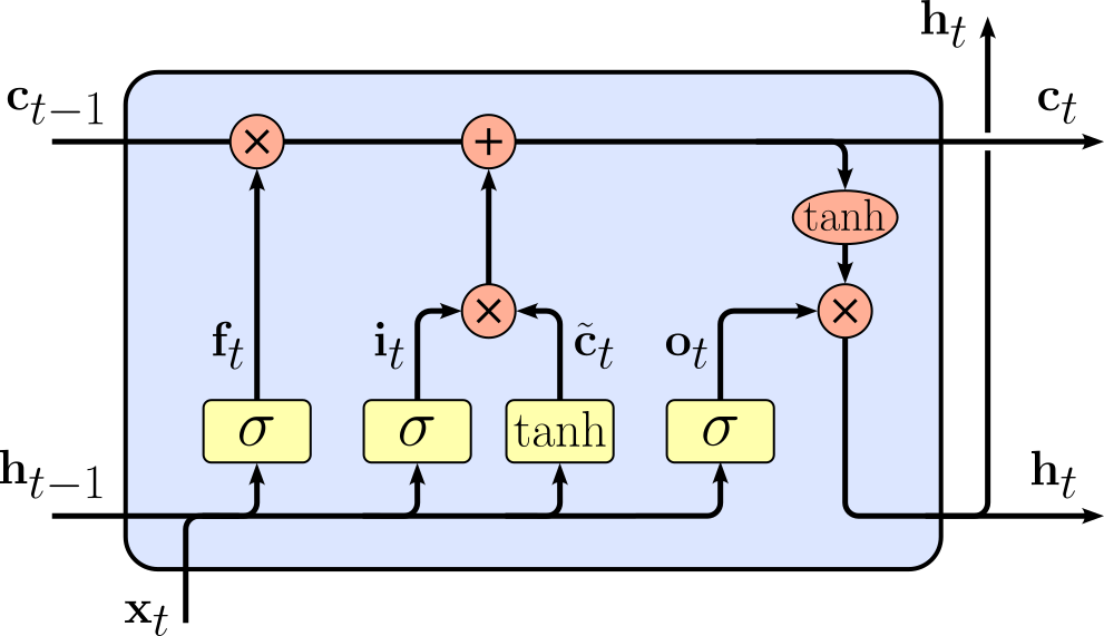
Again, here it is enough to appreciate the recurrence is based on more sophisticated series operations compared to the Vanilla RNN cell. A more detailed introduction into LSTMs is its own topic and beyond the scope of this notebook.
Gated Recurrent Unit (GRU)
Gated Recurrent Unit (GRU) networks were first proposed in 2014 by Kyunghyun Cho, Bart van Merriënboer, Caglar Gulcehre, Dzmitry Bahdanau, Fethi Bougares, Holger Schwenk, and Yoshua Bengio in their paper titled "Learning Phrase Representations using RNN Encoder–Decoder for Statistical Machine Translation". GRUs were introduced as a simpler alternative to Long Short-Term Memory (LSTM) networks, aiming to retain the benefits of long-term dependency learning while reducing computational complexity. While LSTMs use three gates (input gate, forget gate, and output gate) along with a cell state and hidden state, GRUs simplify this mechanism by using only two gates (reset gate and update gate) and maintaining a single hidden state.
The GRU’s reset gate determines how much past information should be forgotten, while the update gate decides how much of the new input should be incorporated into the hidden state. In contrast, LSTMs explicitly separate short-term and long-term memory using a cell state that allows information to flow through many time steps with minimal modification. This extra layer of control in LSTMs makes them more powerful but also computationally more expensive compared to GRUs. Because GRUs have fewer gates and no separate cell state, they are computationally faster and require fewer parameters than LSTMs. This makes GRUs a good choice for real-time applications and when working with limited computational resources. However, LSTMs can sometimes perform better on tasks requiring very long-term dependencies due to their more structured memory management.
For comparison, let's again have a look at visualization of the GRU cell — compared to the LSTM cell and the Vanilla RNN cell.
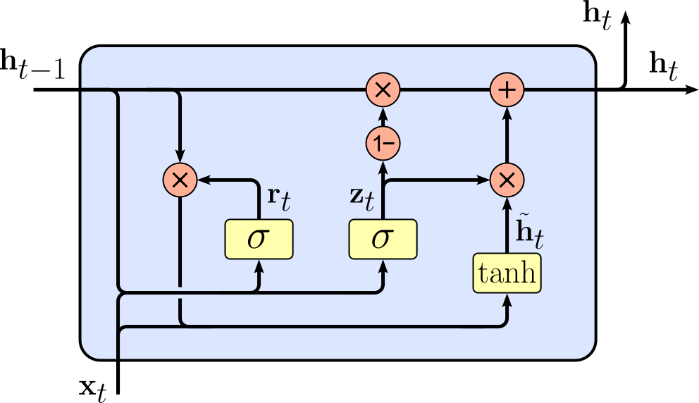
Just from eye-balling this visualization of the GRU cell you can already see the reduced complexity compared to the LSTM cell. However, like for LSTMs, a deeper discussion of GRUs is beyond this notebook's scope but will be covered as its own topic. In conclusion, in practice, LSTMs or GRUs are generally always preferred over Vanilla RNNs given their clear advantages when dealing sequential data.
LSTM cells and GRU cells are not the only variants that have been proposed, but they are the two most popular ones.
Extensions
Apart from the concrete implementation of the recurrent formula in terms of the Vanilla RNN Cell, the LSTM cell, and the GRU cell, Recurrent Neural Networks can also be extended with respect to their over setup. So far we only considered a single hidden layer and the processing of the input sequences from the first input vector to the last input vector in the sequence. Hence, two common extensions refer to the use of multiple hidden layers and the processing of a sequence in both directions to further give the model more capacity to learn. Let's look at the fundamental idea of those two extensions.
Multilayer RNNs
A Multilayer Recurrent Neural Network (RNN) is an extension of a standard RNN where multiple RNN layers are stacked on top of each other. In a standard RNN, there is only a single recurrent layer that processes the input sequence and passes hidden states over time. In contrast, a multilayer RNN has multiple layers of recurrent units, where each layer's output serves as the input to the next layer. This deeper structure allows the model to capture more complex patterns in sequential data by learning hierarchical representations. While more layers add to the model's capacity to learn, stacking multiple layers also increases computational complexity and training difficulty, often requiring techniques like dropout or batch normalization to prevent overfitting. The image below shows an unrolled representation of a 2-layer RNN.
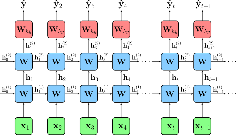
Here, $\mathbf{W}^{(k)}$ denotes to the $k$-th layer, and $\mathbf{h}^{k}_{t}$ denotes the hidden state of the $k$-the layer at time step $t$. In practice, the number of layers in a multilayer RNN typically ranges from $2$ to $4$ layers, though it depends on the complexity of the task and available computational resources. For simpler tasks like basic text classification or small-scale time-series forecasting, $2$ layers are often sufficient — or simply just a single recurrent layer. More complex applications, such as speech recognition or machine translation, may use $3$ to $4$ layers to capture deeper sequential dependencies. However, beyond $4$ layers, improvements often diminish due to increasing training difficulty, vanishing gradients, and computational overhead.
Of course, more than $2$ layers can be stacked upon each other.
Bidirectional RNNs
A Bidirectional Recurrent Neural Network (BiRNN) is a type of RNN that processes input sequences in both forward and backward directions. Unlike a standard RNN, which only has a single hidden state that moves forward in time, a BiRNN consists of two RNN layers — one that processes the sequence from start to end (forward direction) and another that processes it from end to start (backward direction). The outputs of these two layers are then combined, typically through concatenation or summation, to provide a more comprehensive representation of the input sequence. The key advantage of a BiRNN over a standard RNN is its ability to capture both past and future context at each time step. In a standard RNN, predictions at a given time step depend only on past information, which can be limiting in tasks where future context is also important. For example, in speech recognition or language modeling, understanding a word's meaning may depend on both previous and upcoming words in a sentence. However, the trade-off is that BiRNNs require more computation and memory since they process the input twice — once forward and once backward — making them less efficient for real-time applications. The image below illustrates this concept of a BiRNN using the unrolled representation of the network.
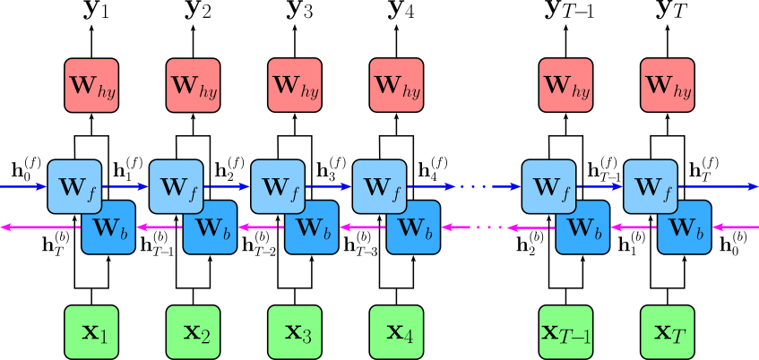
Both directions have their own weight matrices for the input — $\mathbf{W}^{(f)}_{xh}$ and $\mathbf{W}^{(b)}_{xh}$ — as well as for the hidden states — $\mathbf{W}^{(f)}_{hh}$ and $\mathbf{W}^{(b)}_{hh}$; the same is true for the bias vectors $\mathbf{b}^{(f)}_y$ and $\mathbf{b}^{(b)}_h$. Note that $\mathbf{h}^{(b)}_{T+1}$ denotes that initiall hidden state of the backward pass. Each hidden state $\mathbf{h}_t$ is derived from the concatenation of $\mathbf{h}^{(f)}_{t}$ and $\mathbf{h}^{(b)}_{t}$. Using the same recurrent formula as for a Vanilla RNN, the Vanilla BiRNN is therefore implemented as:
Notice that the computation of the hidden state for the backward pass $\mathbf{h}^{(b)}_t$ now relies on $\mathbf{h}^{(b)}_{t+1}$ — instead of $\mathbf{h}^{(b)}_{t-1}$ like for the forward pass. Hence, the notion of $\mathbf{h}^{(b)}_{T+1}$ for the initial hidden state for the backward pass.
Multilayer Bidirectional RNNs
Lastly, we can also combine the idea of multiple layers and the consideration of both directions within the same architecture, where each layer implements both the forward and backward directions. The figure below illustrates the architecture of a $2$-layer BiRNN. Unlike in previous figures the edges are not labeled with the corresponding weight matrices to ease presentation.
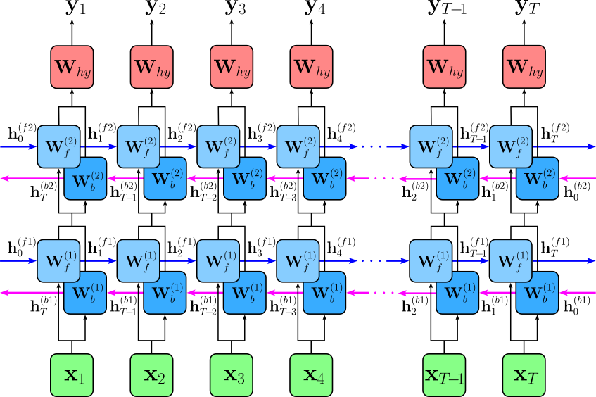
When implementing this $2$-layer BiRNN, we now have to distinguish between both the layer and the direction for each hidden state, weight matrix, and bias vector. The first bidirectional layer is therefore implemented as follows; again, we get the final output of the first layer $\mathbf{h}^{(1)}_t$ by concatenating the individual outputs for both directions.
The second layer is implemented exactly the same, only taking $\mathbf{h}^{(1)}_t$ as its input.
And as before, we get the final output $\mathbf{\hat{y}}_t$ as
Like for unidirectional RNNs, it is easy to see how this implementation can be extended to more than $2$ layers. In general, stacking multiple recurrent layers in an RNN increases the model's capacity to learn complex patterns in sequential data. In both unidirectional and bidirectional RNNs, deeper architectures enable the model to capture richer temporal dependencies and interactions within the data.
However, increasing the number of layers also increases the overall complexity of the model. Each additional recurrent layer introduces new parameters and additional computations during both the forward pass and backpropagation through time. This raises the computational cost and memory requirements, and can make training more difficult due to issues such as vanishing or exploding gradients. As a result, deeper RNN architectures can become harder to optimize and more prone to overfitting if not carefully regularized. In practice, adding many recurrent layers often yields only limited performance improvements. While a small number of stacked layers can help the model learn more expressive sequence representations, the marginal benefit typically diminishes as depth increases. Consequently, many practical RNN architectures use only a few recurrent layers, balancing representational power with computational efficiency and training stability.
Discussion & Limitations
While Recurrent Neural Networks represent a powerful extension to basic Feed-Forward Neural Networks to support the processing of sequences, they also introduce new challenges. In a nutshell, these challenges more or less all derive from the sequential nature of Recurrent Neural Networks, particularly when dealing with long sequences.
Performance Consideration
Recurrent Neural Networks (RNNs) process input data sequentially, meaning that each step depends on the computation of the previous step. This strict sequential processing creates a significant bottleneck in terms of performance, especially when dealing with long sequences. Unlike feedforward neural networks, where computations can be parallelized, RNNs must process each time step one after another, making them inherently slower, particularly for long sequences in tasks like natural language processing (NLP) or time-series analysis.
One major issue with this sequential dependency is that it prevents efficient parallelization on modern hardware, such as GPUs and TPUs, which thrive on executing multiple operations simultaneously. In contrast, architectures like Transformers leverage mechanisms such as self-attention, allowing computations to be performed in parallel, greatly improving efficiency. Because of this limitation, RNNs are often significantly slower in training and inference compared to newer deep learning architectures.
Training Challenges
The problem with long-term dependencies in training RNNS arises from the difficulty of propagating information across many time steps. Ideally, RNNs should be able to capture patterns and relationships in sequences, even when important information appears far back in the input. However, due to the way gradients during training, long-range dependencies are often lost or distorted:
One major issue is the vanishing gradient problem, where gradients become extremely small as they are propagated backward through many time steps. When this happens, earlier layers receive almost no updates, making it difficult for the model to learn relationships between distant time steps. As a result, the network becomes biased toward recent inputs and struggles to remember important information from the past, which is crucial for tasks like speech recognition, machine translation, and time-series forecasting.
Conversely, RNNs can also suffer from the exploding gradient problem, where gradients grow exponentially large, causing instability in training. This can lead to wildly fluctuating weight updates, making it difficult for the network to converge. While techniques like gradient clipping can help control exploding gradients, the vanishing gradient problem remains a more persistent challenge for capturing long-term dependencies.
To address these issues, architectures like Long Short-Term Memory (LSTM) networks and Gated Recurrent Units (GRUs) were developed. These models introduce gating mechanisms that regulate how information is stored, forgotten, and passed forward through time, helping preserve long-term dependencies. However, even with these improvements, RNNs still struggle with long sequences, which is why attention-based models like Transformers have largely replaced them in many applications.
Information Bottleneck
Recall the basic encoder-decoder setup used for tasks such as machine translation where we use an encoder RNN to process the an sequence in the source language and use the final hidden state of the encoder RNN to initialize the hidden state of the decoder RNN:
In simple terms, this setup assumes that the last hidden state of the encoder RNN has sufficiently captured the meaning of the input sentence — otherwise we could not meaningfully expect the decoder RNN to generate the appropriate translation in the target language. This means that the encoder processes the input sequence one step at a time and condenses all the information into a single vector, often called the context vector or bottleneck vector. The decoder then relies entirely on this vector to generate the output sequence. This design creates several challenges, particularly when dealing with long or complex sentences:
Firstly, compressing all the relevant information into a single vector can lead to information loss. If the input sentence is long or contains multiple important details, the encoder may struggle to retain all necessary information, causing the decoder to generate inaccurate or incomplete translations. This is especially problematic for languages with different word orders or complex grammatical structures, as the decoder might lack sufficient context to reconstruct a coherent output.
Secondly, long-range dependencies become harder to capture. Since RNNs already struggle with vanishing gradients when processing long sequences, the encoder may fail to retain information from the beginning of a long sentence, making it difficult for the decoder to correctly interpret or generate a response based on earlier words.
To overcome these limitations, attention mechanisms were introduced. Instead of relying on a single context vector, attention allows the decoder to access different parts of the encoder's hidden states at each time step, dynamically focusing on relevant words. This improvement has led to significant advancements in machine translation, ultimately paving the way for models like the Transformer, which entirely replace RNNs with more efficient self-attention mechanisms.
Summary & What's Next?
Recurrent Neural Networks (RNNs) are a class of artificial neural networks designed to process sequential data by maintaining a memory of previous inputs. Unlike traditional feedforward neural networks, which treat each input independently, RNNs introduce a recurrent connection that allows information to persist across time steps. This makes them well-suited for tasks involving sequences, such as natural language processing (NLP), speech recognition, and time-series forecasting.
The core concept of an RNN lies in its hidden state, which acts as a form of memory that carries information from previous time steps to the current computation. At each step, the RNN updates its hidden state based on both the current input and the previous hidden state. However, standard RNNs struggle with long-term dependencies due to the vanishing gradient problem, which makes it difficult for the network to retain information over long sequences. To address these challenges, advanced RNN architectures such as Long Short-Term Memory (LSTM) networks and Gated Recurrent Units (GRUs) were developed. These models introduce gating mechanisms that help regulate information flow, allowing them to retain important information for longer periods. As a result, LSTMs and GRUs have significantly improved the performance of AI applications in areas like machine translation, sentiment analysis, and speech synthesis.
RNNs play a crucial role in AI and machine learning by enabling models to understand and generate sequential data, making them essential for human-computer interaction and automation. While more recent models like Transformers have gained popularity due to their efficiency in handling long sequences, RNNs remain foundational in the study of deep learning for sequential tasks. Their ability to model time-dependent patterns continues to make them valuable in fields such as healthcare, finance, and robotics.
In this notebook, we covered the basic idea behind Recurrent Neural Network by extending basic Feed-Forward Neural Neural giving the network a "memory" represented by the hidden state. We see how the introduction of this hidden state and the recurrent formula to update the hidden change now allows the processing of sequential data such as natural language texts, time series data, or audio and video data. Other notebooks will delve deeper into the implementation and training of RNNs; important topics include:
Backpropagation Through Time (BPTT). In principle, RNNs are trained using backpropagation like most other neural network architectures. However, the involved recurrence adds complexity to this task. BPTT is the adaptation of the standard backpropagation algorithm for training Recurrent Neural Networks (RNNs). Since RNNs process sequential data, they have connections that span multiple time steps. Unlike Feed-Forward Neural Networks (FNNs), where information flows in one direction and errors are backpropagated layer by layer, RNNs unroll across time steps, and errors are backpropagated through each time step sequentially. This means that during training, BPTT computes gradients not only across layers (as in standard backpropagation) but also across time, making the process computationally more intensive.
RNNs with Attention. The idea of attention in Recurrent Neural Networks is to allow the model to focus on different parts of the input sequence dynamically, rather than relying on a single fixed-length context vector. Traditional RNN-based encoder-decoder models for tasks like machine translation compress all input information into a single context vector, which can become a bottleneck, especially for long sentences. Attention mechanisms solve this problem by enabling the decoder to selectively "attend" to different parts of the input sequence at each decoding step. The attention mechanism works by computing a set of weights that determine how much focus should be given to each encoder hidden state when generating each output token. Instead of relying on a single compressed representation, the decoder can look at different parts of the input sequence as needed. This significantly improves performance in tasks where understanding long-range dependencies is important, such as machine translation, speech recognition, and text summarization.
Practical Applications. In this notebook, we have introduced Recurrent Neural Networks on a fairly high level, focusing on their core ideas and how RNNs are — at least, in principle — are capable of handling a wide range of sequence tasks. As such, this notebook alone is unlikely to help much when it comes to actually training RNNs on real-world datasets. Actually training RNNs also helps to actually appreciate the challenges when working with RNNs. These challenges include not only those outlined above, but also very pragmatic challenges. For example, when working with batches, most implementations of RNNs assume that all sequences in a batch have the same length. Assuming our input are natural language sentences, our input sequences are likely to have different lengths. We need to see how such constraints are commonly met in practice.
All the topics and techniques will be covered in detail in separate notebooks.