Disclaimer: This Jupyter Notebook contains content generated with the assistance of AI. While every effort has been made to review and validate the outputs, users should independently verify critical information before relying on it. The SELENE notebook repository is constantly evolving. We recommend downloading or pulling the latest version of this notebook from Github.
RNN-based Language Models
Recurrent Neural Networks (RNNs) were once the dominant architecture for natural-language generation and sequence modeling, playing a crucial role in the evolution of modern deep learning. While they have largely been surpassed by Transformers, RNNs remain extremely valuable for learning how sequential models work at a fundamental level. In this notebook, we will train an RNN-based language model (specifically an LSTM) from scratch using PyTorch. The goal is not to build a state-of-the-art system but to understand each step of the process, from preparing the data to building the model and performing backpropagation through time (BPTT).
To keep the focus on the concepts rather than computational complexity, we will train on a dataset of 100,000 movie reviews. This dataset is large enough to expose the real-world challenges of training sequence models — such as handling long sequences, learning useful token representations, and managing hidden states — yet small enough to allow fast experimentation on standard hardware. Working with a text corpus of this size provides a realistic demonstration of issues that arise when scaling RNNs, such as vanishing gradients, limited long-range memory, and the need for truncated BPTT.
RNNs process text one time step at a time while maintaining a hidden state that is passed forward through the sequence. This sequential processing makes them intuitive to understand but also highlights their major limitations. Training is inherently slow due to the lack of parallelism, and long-range dependencies are difficult to capture because the hidden state must compress everything seen so far. These difficulties are exactly what motivated the development of the Transformer architecture, which replaces recurrence with attention, enabling full parallelism and more effective learning of long-distance relationships.
By building an LSTM language model from the ground up, you will gain a deeper appreciation of how sequence models operate internally and why training them can be challenging. Understanding these limitations provides essential context for understanding why Transformers became the standard for NLP and why architectural shifts were necessary. Throughout the notebook, we will focus on clarity, practical implementation decisions, and conceptual insight rather than model performance, making the learning process both accessible and grounded in real-world considerations.
If you are ready, we can continue to the dataset preparation section or outline the full training pipeline.
Setting up the Notebook
Make Required Imports
This notebook requires the import of different Python packages but also additional Python modules that are part of the repository. If a package is missing, use your preferred package manager (e.g., conda or pip) to install it. If the code cell below runs with any errors, all required packages and modules have successfully been imported.
import os, sys
import numpy as np
from tqdm import tqdm

import torch.nn as nn
import torch.optim as optim
import torch.nn.functional as F
from torch.utils.data import Dataset, DataLoader, IterableDataset

from transformers import AutoTokenizer

from src.utils.compute.gpu import *
from src.utils.data.files import *
Download Required Data
Some code examples in this notebook use data that first need to be downloaded by running the code cell below. If this code cell throws any error, please check the configuration file config.yaml if the URL for downloading datasets is up to date and matches the one on Github. If not, simply download or pull the latest version from Github.
movie_reviews_zip, target_folder = download_dataset("text/corpora/reviews/movie-reviews-imdb.zip")
File 'data/datasets/text/corpora/reviews/movie-reviews-imdb.zip' already exists (use 'overwrite=True' to overwrite it).
We also need to decompress the archive file.
movie_reviews = decompress_file(movie_reviews_zip, target_path=target_folder)

print(movie_reviews)
['data/datasets/text/corpora/reviews/movie-reviews-imdb.txt']
Checking & Setting Computing Device
PyTorch allows to train neural networks on supported GPU to significantly speed up the training process. If you have a support GPU, feel free to utilize it. However, for this notebook it's certainly not needed as our dataset is small and our network model is very simple. We provide an auxiliary method to automatically select the best device. It checks if a supported GPU is available and if so, uses it as the preferred device.
# Select preferred device (GPU, if available; CPU otherwise); you can enfore the use of the CPU
DEVICE = select_device(force_cpu=False)

print("Available device: {}".format(DEVICE))
Available device: cuda:0
Preliminaries
Before checking out this notebook, please consider the following:
This notebook is for education and not to build a state-of-the-art LLM. Not only is the dataset very small it also stems for a single domain: movie reviews. We also use a rather simple RNN-based model to keep things simple and reasonably fast. In any case, do not expect human-like responses from the trained model, particularly in demo mode (see below).
We assume that you have a good understanding of RNNs in general. If not, we have a notebook that provides an introduction to Recurrent Neural Networks.
While not strictly required, we recommend the presence of a GPU to speed up the training. However, any more modern consumer GPU supported by the PyTorch library should be fine. Even for the full training mode, the default parameters are chosen that the training will not require more than 10 GB of VRAM; with 16GB slowly becoming the standard even for consumer GPUs.
You can run the notebook in demo mode by using
mode = "demo"in the code cell below. In demo mode, we only use 10,000 out of the 100,000 movie reviews. We recommend first using the demo mode to see how long the training of the model for individual epochs will require.
mode = "demo"
#mode = "full"
Dataset Preparation
The ACL IMDB (Large Movie Review) dataset is a popular benchmark dataset for sentiment analysis, introduced by Andrew Maas et al. (2011). It contains a total of 100,000 movie reviews collected from IMDb, with 50,000 reviews being labeled as either positive or negative and evenly split into 25,000 reviews for training and 25,000 for testing. For training Word2Vec word embeddings we do not need the sentiment labels. We therefore already preprocessed the original dataset such that all 100,000 reviews are in a single file, with 1 line = 1 review. This preprocessing included the removal of any HTML tags and line breaks.
For the training of our model, we make the common assumption that the training data is structured as continuous streams of documents, with each movie review representing a document. Document streams refer to the way text data is fed into the model during training: not as isolated documents, but as a continuous stream of text. Instead of treating each document as an independent unit, the training corpus is viewed as a long sequence of tokens coming from many documents concatenated together. This approach allows the model to learn language patterns and long-range dependencies across boundaries that would otherwise be artificially imposed by document splits. The training process still ensures that context resets appropriately between documents (e.g., by inserting special end-of-document tokens [EOS]), but from the model's perspective, the data flows in a seamless stream. Thus, assuming $\text{doc}_{i}$ is a list of tokens represents the $i$-th documents, our document stream has the following format:
In practice, our training data may consist of many such document streams so that each stream can fit into memory. However, here we work with a small example data for educational purposes. This includes that the stream of tokens can be represented by an array that fits completely into memory, therefore avoiding any more sophisticated strategies requiring the splitting of the dataset, etc.
Document streaming is essential for efficient batching and scaling when training on massive corpora. LLMs are typically trained on trillions of tokens spread across billions of documents, and it's computationally impractical to load entire documents or reinitialize contexts for each. Instead, data pipelines tokenize all documents in advance, concatenate them, and then dynamically sample fixed-length chunks (e.g., 1024 tokens) to feed into the model. This "streaming" setup keeps GPUs fully utilized and allows distributed training systems to continuously stream data without needing to restart or reshuffle individual documents frequently.
Load Reviews from File
In the setup section of the notebook, we already downloaded the file containing all 100,000 movie reviews. In the following code cell, simply counts the number of reviews by containing the number of each line in the file, just to check if the dataset is complete. Note that we have to write movie_reviews[0] since movie_reviews is a list of files — it just so happens that the list contains only one file.
total_reviews = sum(1 for _ in open(movie_reviews[0]))

print(f"Total number of reviews (1 review per line): {total_reviews}")
Total number of reviews (1 review per line): 100000
Although we have a total 100,000 reviews (each containing multiple sentences), we consider only 10,000 reviews in demo mode to speed up the training. However, you can edit the code cell below to increase or decrease the number of considered reviews. For a first run, we recommend sticking to 10,000 reviews to execute and understand the code.
if mode == "demo":
    num_considered_reviews = 10_000
else:
    num_considered_reviews = 100_000

num_reviews = min(total_reviews, num_considered_reviews)

print(f"Number of reviews used for training dataset: {num_reviews}")
Number of reviews used for training dataset: 10000
Tokenize & Generate Token Stream
Early RNN-based language models were typically trained on word-level vocabularies. Each word was treated as an atomic symbol with its own embedding, which made the models simple to conceptualize and train. However, this approach came with significant drawbacks. Word vocabularies must be extremely large to cover real text, often reaching hundreds of thousands of tokens, which dramatically increases memory requirements. More importantly, word-based models cannot naturally handle unseen or rare words, forcing them into a generic <unk> (unknown) token that discards important information and weakens the model's ability to generalize.
Over time, subword tokenization such as Byte Pair Encoding (BPE), SentencePiece, or WordPiece became the standard for modern language models, including Transformer-based systems. Subword vocabularies strike a balance between characters and words: they are small enough to be efficient, yet expressive enough to represent any word by composing smaller units. This eliminates the <unk> problem entirely, improves handling of rare and morphologically rich words, and reduces vocabulary size dramatically, which helps models train more efficiently.
For RNN-based models, subword tokenization offers the same advantages: fewer out-of-vocabulary issues, smaller embeddings, and more robust representations of linguistic structure. While RNNs were not originally trained this way due to computational limitations and tooling complexity at the time, subword units now provide a more scalable and practical foundation for any neural language model, regardless of architecture.
This is why we will be using subword tokenization in this notebook by means of a pretrained tokenizer. More specifically, we are using GPT-2 tokenizer to handle both the tokenization and indexing for us. The GPT-2 tokenizer is a subword tokenizer based on the Byte-Pair Encoding (BPE) algorithm. In nutshell, BPE (and similar approaches) learns how to tokenize words from data. Instead of splitting text strictly into full words or individual characters, BPE breaks words into frequently occurring subword units. For example, "unhappiness" might become "un", "happi", and "ness". This enables the model to represent common words as single tokens while decomposing rare words into smaller, reusable pieces, preventing the out-of-vocabulary (OOV) problem that word-level tokenizers suffer from. Because subword tokens capture meaningful morphological patterns (prefixes, suffixes, roots), models can infer the meaning of new or compound words based on familiar subparts. This reduces the total number of parameters needed for embeddings and improves the model's ability to generalize to unseen text. You can learn all about BPE in a separate notebook
To load the pretrained GPT-2 tokenizer, we can use the AutoTokenizer class Hugging Face Transformers library. This class is a high-level interface that automatically selects the appropriate tokenizer for a given pretrained model, abstracting away the need to know the specific tokenizer class. The from_pretrained method is used to load a tokenizer that has already been trained on a specific model's vocabulary and tokenization rules, either from the Hugging Face model hub or a local path. This method ensures that the tokenizer is configured consistently with the pretrained model, including token-to-ID mappings, special tokens, and any subword tokenization schemes (e.g., BPE), making it ready for encoding text into token IDs suitable for model training or inference. The code cell below used the class and method to load the GPT-2 tokenizer.
tokenizer = AutoTokenizer.from_pretrained("gpt2")
Recall that for our document stream, we need to indicate when one movie review ends and another review starts using some [EOS] (end-of-sequence) token. However, we cannot simply define our own unique token but must use a token that is known to the tokenizer, i.e., the token is part of the existing vocabulary. Most tokenizers include a small set of special tokens to indicate the end of a sequence, the beginning of a sequence, padding tokens, masked tokens, etc. — all depending on the data and learning task.
We can check the special_tokens_map of the GPT-2 tokenizer which special tokens it supports:
tokenizer.special_tokens_map
{'bos_token': '<|endoftext|>',
 'eos_token': '<|endoftext|>',
 'unk_token': '<|endoftext|>'}
We can see that the GPT-2 tokenizer recognizes only one special token: <|endoftext|>. Since GPT-2 was also trained on a document stream, we only need a single token acting as a separator between documents, which could be either the [EOS] or [BOS] token. The GPT-2 tokenizer also does not require a dedicated [UNK] (unknown) token, since BPE just tokenizes unknown words into known subwords or even just characters, if needed.
Let's define this <|endoftext|> token as a constant for creating our document stream. Using the tokenizer instance, we can also encode this special token to get its unique index. We will need this index later when generating text using our RNN-based language model.
EOS_TOKEN = "<|endoftext|>"
EOS_TOKEN_INDEX = tokenizer.encode(EOS_TOKEN)[0]
With the tokenizer, we can now go through all movie reviews (or the maximum number of reviews specified) and tokenize them; see the code cell below. Notice that the preprocess each review before tokenizing by removing any newline characters, converting all words to lowercase, and adding the special [EOS] token at the end.
Lowercasing all words can be very useful when working with smaller datasets because it significantly reduces the size of the vocabulary the model needs to learn. In a small corpus, many words appear only a handful of times, and treating uppercase and lowercase forms as separate tokens (e.g., "Movie" vs. "movie") further fragments the data. By converting everything to lowercase, the model encounters each word more frequently, allowing it to learn better embeddings and stronger statistical patterns from limited examples. This makes training more stable and reduces the risk of overfitting to infrequent capitalized variants.
Additionally, the goal in many educational or exploratory projects is to understand the mechanics of training sequence models and not to capture subtle linguistic nuances such as proper noun capitalization. Lowercasing simplifies preprocessing, reduces noise, and helps the model focus on learning the core structure of the language rather than expending capacity on orthographic variations. For small-scale experiments, this trade-off is highly beneficial: you get cleaner data, faster training, and more reliable results without sacrificing the insights the project aims to teach.
tokens = []

with open(movie_reviews[0]) as file:
    for idx, review in enumerate(tqdm(file, total=num_reviews, leave=False)):
        if idx >= num_reviews:
            break
        tokens.extend(tokenizer.encode(f"{review.strip().lower()} {EOS_TOKEN}", truncation=True, max_length=sys.maxsize))

print(f"Total number of tokens: {len(tokens)}")
Total number of tokens: 2922984
Create Dataset and DataLoader
PyTorch's Dataset class provides a clean and modular way to represent and access your data. It allows you to define how individual samples are loaded, whether they come from tokenized text, images on disk, or preprocessed tensors. This abstraction keeps the data logic separated from the model and training loop, making your code easier to maintain and allowing you to swap in different datasets without changing the rest of your pipeline. The DataLoader builds on top of a Dataset to efficiently feed data to the model during training. It handles batching, shuffling, and parallel data loading through worker processes, which significantly speeds up training and keeps the GPU fully utilized. Together, Dataset and DataLoader provide a flexible and scalable framework for handling data in PyTorch, allowing you to focus on model design and experimentation rather than manually managing data batching or iteration logic.
Batching Considerations
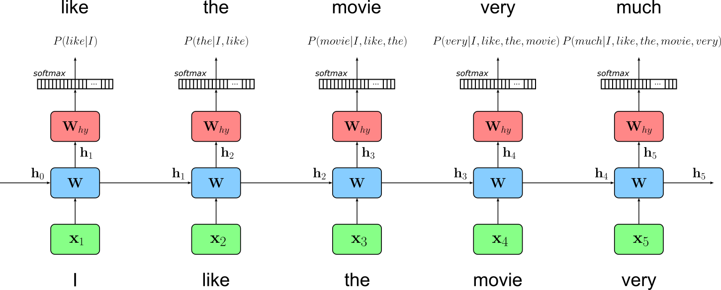
Like most language models, RNN–based language models are motivated by the need to capture sequential dependencies in language, where the meaning of each word often depends on the words that came before it. Because natural language is inherently ordered, RNNs process text one token at a time, updating an internal hidden state that summarizes everything seen so far. To train such models to understand and generate coherent text, they are typically optimized using the next-word prediction task: given a sequence of input tokens, the model must predict the next token at every time step. This setup naturally encourages the model to learn patterns of grammar, vocabulary, and long-range dependencies.
In this training objective, the target sequence is simply the input sequence shifted one position to the left. For example, if the input is "I like the movie very", the model is trained to predict "like the movie very much"; this figure below illustrates this idea. This formulation is elegant and powerful because it directly aligns the model's predictions with the structure of language, making it possible for the model to learn how each word follows from its preceding context. Through repeated exposure to large corpora, the RNN becomes able to generate fluent text by repeatedly applying this next-word prediction ability.
In principle, we could feed our continuous stream of tokens to the RNN. However, RNNs are typically restricted in maximum sequence length because their ability to preserve information over time degrades as sequences grow longer. During training, gradients must be propagated backward through every time step, and this repeated multiplication can cause them to vanish or explode. Vanishing gradients make it difficult for the model to learn long-range dependencies, while exploding gradients can destabilize training altogether. Although variants like LSTMs and GRUs mitigate these issues with gating mechanisms, they still struggle when sequences become very long.
Furthermore, longer sequences also increase computational cost and memory usage, since the hidden state and gradients for every time step must be stored during training. This limits the practical maximum sequence length that can be processed efficiently on modern hardware. As a result, even though RNNs are theoretically capable of handling arbitrarily long sequences, in practice they perform best when trained on moderately sized segments that balance computational feasibility with the ability to capture meaningful context. We therefore need to split our token stream into fixed-size chunks and pass the chunks to the model during training
To maximize training efficiency, we also do not want to pass single chunks but batches containing more than one chunk in one training step. A naive approach would be to treat each chunk independently and reset the hidden state for each batch of chunks. However, treating each batch independently and resetting the hidden state at every batch boundary prevents the model from carrying information across sequence segments. Since RNNs rely on their hidden state to encode contextual information from previous tokens, resetting it means the model "forgets" everything it has learned about the text up to that point. This effectively breaks the continuity of the training data and prevents the model from learning dependencies that span beyond the fixed sequence length used in each batch.
As a result, the model only learns relationships within individual segments rather than across the natural flow of the corpus. This can significantly weaken its ability to model long-range structure (such as topic shifts, document-level coherence, or dependencies spanning many sentences) because the hidden state is never allowed to accumulate context over longer stretches of text. For this reason, some training approaches like truncated backpropagation through time (TBPTT) maintain hidden states across batches within the same sequence stream, allowing the RNN to capture longer-term patterns while still keeping training manageable.
To organize our dataset to properly support TBPTT, we have to make sure that the $k$-th chunk in the $i$-th batch is a continuation of the $k$-th chunk in the $(i\!-\!1)$-th batch. To illustrate this, let's assume that our token stream contains the token $1$ to $60$ as shown below:
[1, 2, 3, 4, 5, 6, 7, 8, 9, 10, 11, 12, 13, 14, ..., 57, 58, 59, 60]
The idea is now to split the single token stream into multiple streams with the batch_size determining the number of substreams. Then, when forming a batch of sequences of length seq_len, we move a sliding window (with no overlap) of size seq_len across all substreams, resulting in batch of shape (batch_size, seq_len) that is also a continuation of the previous batch (apart from the first batch, of course). The figure below visualizes this idea using our simple example of $60$ tokens in the initial token stream. In this example, we assume a batch size of $3$, resulting in $3$ substreams.
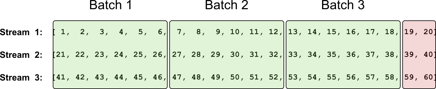
Notice that the last tokens (indicated by the red box in the figure above) do not form a complete batch with sequences of length seq_len. Although an RNN can work with sequences of arbitrary lengths, keep in mind that for this last reduced batch, we are no longer able to generate the target sequences after shifting the input sequence $1$ token to the left. Although we could fill the "missing" places with the [EOS] token, we can also simply ignore this batch. When working with large datasets with millions of tokens or more, dropping a few sequences does not matter at all.
Implementing Custom DataSet Class
Now that we know in which format we have to bring our training data, we can implement a custom DataSet to achieve this. More specifically, create a class that inherits from the IterableDataset class. This dataset class is designed for scenarios where data must be generated or streamed sequentially rather than randomly accessed. Unlike the standard Dataset class, which assumes that individual samples can be indexed (__getitem__()), an IterableDataset only requires the implementation of an __iter__() method that yields data samples one at a time. This makes it ideal for use cases such as reading data from large text files, streaming logs, or generating data on the fly—situations where random access is impossible or inefficient.
Because IterableDataset produces samples in a fixed order, it gives the user precise control over the data flow, which is especially useful for tasks like language modeling with long text streams, reinforcement learning, or online learning. However, this sequential nature also means that certain DataLoader features (e.g., shuffling or automatic batching) are limited or behave differently. This includes that we have to implement batching ourselves — but we know how to do it (see the figure above). Despite these constraints, IterableDataset is a powerful tool when working with continuous or very large datasets that don't fit neatly into memory or require sequential processing.
The class StreamDataset in the code cell below implements the approach. When passing the initial array of tokens, the batch_size, and the sequence length seq_len of all sequences within a batch, the constructor performs the following three main steps:
(1) Compute the number of usable tokens: This step refers to ignoring the last tokens in each substream which are insufficient to form a full batch. We can compute this number by first computing the number of full batches by dividing the total number of tokens by the batch size using an integer division (without remainder). The number of usable tokens is the number of batches, and then multiplied again by the number of batches.
(2) Create substreams: We can create all batch_size substreams by reshaping the original 1-dim array of tokens into a 2-dim array of shape (batch_size, stream_len) where stream_len is the number of tokens in each substream — this number is, of course, the number of usable tokens divided by the batch size (i.e., the number of streams). Having all streams in a single array makes creating the final batches very easy.
(3) Compute total number of batches: Even if now the last batch is guaranteed to be full (i.e., all sequences have a length of seq_len) we still want to ignore it since we still could not generate the target sequences by shifting the inputs sequences $1$ token to the left — again, we could add an [EOS] token but we simply do not have to. Thus, to get the final number of batches, we simply use an integer division to divide the lengths of the streams $-1$ by seq_len.
In the __iter__() method simply iterate overall valid batches numbers (i.e., their index from 0 to n_batches-1) to generate all input sequences and target sequences by slicing the 2-dim array that holds all substream. Notice the +1 as part of the slicing for the target sequences. This implements the shifting of the tokens by $1$ token to the left.
class StreamDataset(IterableDataset):

    def __init__(self, tokens: torch.LongTensor, batch_size: int, seq_len: int):
        super().__init__()
        self.tokens = tokens
        self.batch_size = batch_size
        self.seq_len = seq_len
        # (1) Compute number of usable tokens
        total_tokens = tokens.size(0)
        usable = (total_tokens // batch_size) * batch_size
        self.tokens = tokens[:usable].contiguous()
        self.stream_len = usable // batch_size  # length of each stream
        # (2) Create substreams: reshape into (batch_size, stream_len)
        self.streams = self.tokens.view(batch_size, self.stream_len)
        # (3) Compute total number of batches: ignore the last batch, even if it is full
        self.n_batches = (self.stream_len - 1) // self.seq_len

    def __iter__(self):
        s = self.seq_len
        # Generate next pair of inputs and targets
        for step in range(self.n_batches):
            inputs = self.streams[:,(step*s):(step*s+s)]
            targets = self.streams[:,(step*s+1):(step*s+s+1)]
            yield inputs, targets
To show how it works, we can replicate the example as visualized in the figure about. In the code cell below, we first create a 1-dim array with the numbers from $1$ to $60$. We use this array to create a StreamDataset instance, assuming a batch size of $4$ and a sequence length per batch of $6$.
demo_tokens = torch.arange(1, 61)

demo_dataset = StreamDataset(demo_tokens, batch_size=3, seq_len=6)
To easily iterate over all batches, we first create a DataLoader instance using our demo dataset as input. Since the batching is handled by the StreamDataset class, and we can use shuffling — otherwise we would break the continuation between batches, we basically only pass the dataset instance to the data loader class. Lastly, we can use the data loader to easily iterate over all batches; and print them shown below.
demo_loader = DataLoader(demo_dataset, batch_size=None)

for step, (inputs, targets) in enumerate(demo_loader):
    print(f"========== Batch {step+1} ==========")
    print(f"Input sequences:\n{inputs}")
    print(f"Target sequences:\n{targets}\n")
========== Batch 1 ==========
Input sequences:
tensor([[ 1,  2,  3,  4,  5,  6],
        [21, 22, 23, 24, 25, 26],
        [41, 42, 43, 44, 45, 46]])
Target sequences:
tensor([[ 2,  3,  4,  5,  6,  7],
        [22, 23, 24, 25, 26, 27],
        [42, 43, 44, 45, 46, 47]])

========== Batch 2 ==========
Input sequences:
tensor([[ 7,  8,  9, 10, 11, 12],
        [27, 28, 29, 30, 31, 32],
        [47, 48, 49, 50, 51, 52]])
Target sequences:
tensor([[ 8,  9, 10, 11, 12, 13],
        [28, 29, 30, 31, 32, 33],
        [48, 49, 50, 51, 52, 53]])

========== Batch 3 ==========
Input sequences:
tensor([[13, 14, 15, 16, 17, 18],
        [33, 34, 35, 36, 37, 38],
        [53, 54, 55, 56, 57, 58]])
Target sequences:
tensor([[14, 15, 16, 17, 18, 19],
        [34, 35, 36, 37, 38, 39],
        [54, 55, 56, 57, 58, 59]])
Appreciate how the input sequences match the example batches in the figure above.
Of course, we do not want to train our model based on this demo dataset but on our movie reviews. So let's create a data loader using our initial document stream tokens with a batch size of $256$ and a sequence length of $32$. When training an RNN-based language model on a small dataset, shorter sequences are recommended because they reduce the risk of overfitting and make the learning problem more manageable. With limited data, long sequences can cause the model to memorize specific patterns rather than generalize, since the model repeatedly sees the same long contexts during training. Shorter sequences encourage the model to focus on more frequent, broadly useful local dependencies rather than rare long-range ones that the dataset cannot reliably support.
Shorter sequences also reduce computational load and stabilize training. RNNs struggle with long-term dependencies due to vanishing gradients, and this issue becomes more pronounced when the amount of training data is small. By keeping sequence lengths short, gradients propagate more reliably, batches become more diverse, and the model tends to learn cleaner statistical patterns from the available data.
dataset = StreamDataset(torch.LongTensor(tokens), batch_size=256, seq_len=32)

loader = DataLoader(dataset, batch_size=None)
Keep in mind that creating the dataset and data loader was rather straightforward since the dataset is small enough to easily fit into memory. In contrast, large training datasets typically cannot fit into main memory all at once. Thus, when working with extensive text corpora (often gigabytes in size) loading everything upfront would exceed memory limits. Instead, the data must be streamed, read in chunks, or processed on the fly. This requires dataset implementations that can efficiently iterate through the data without holding it entirely in memory. Because of these constraints, additional considerations are needed when creating Dataset and DataLoader instances. For example, one may extend IterableDataset implementation to read from large text files line by line, implement custom buffering strategies, or perform on-demand tokenization. However, these consideration go beyond the scope of this notebook and are not needed here.
Auxiliary Methods
For the model training and the very crude qualitative evaluation of the model (discussed later), we next define a few auxiliary models for a cleaner code but also support strategies such as checkpointing for training large models in practice.
Training a Single Epoch
As the name suggests, the method train_epoch() trains a given model for one epoch. Apart from the model itself, the method also gets a data loader instance to iterate over all batches, as well as an optimizer to handle the update of the model weights after the gradients have been computed during backpropagation; the description is merely to annotate the progress bar.
Worth mentioning is the hidden variable that holds the hidden state of the RNN model. At the beginning of the hidden epoch, the hidden state is initialized with all zeros. In the loop, when each batch is passed to the model, the hidden states gets updates but not reset. When training an RNN with stateful or continuation batches (i.e., where the hidden state from the previous batch is reused for the next), the hidden state must be detached to prevent gradients from propagating endlessly through the entire training history. Without detach(), PyTorch treats the hidden state as part of the computational graph and keeps linking new operations onto that graph at every step. This causes the graph to grow without bound, dramatically increasing memory usage and eventually causing the training process to crash or slow down severely.
Detaching the hidden state tells PyTorch: "Use the numerical value of this tensor, but treat it as a constant for future gradient computations". In effect, it cuts the backpropagation path so that gradients only flow through the current unrolled sequence length, not through previous batches. This keeps training efficient, bounded in memory, and still allows the RNN to keep its stateful behaviour across batches without unintentionally backpropagating across the entire dataset. In simple terms, without detaching the hidden state, the model would require more and more memory and would trains slower and slower over time.
def train_epoch(loader, model, optimizer, description):
    model.train()

    epoch_loss = 0.0
    device = next(model.parameters()).device
    # Initialize the hidden state
    hidden = model.init_hidden(batch_size=dataset.batch_size, device=device)

    for idx, (inputs, targets) in enumerate(tqdm(loader, desc=description, leave=False, total=dataset.n_batches)):
        # Move data to the same device as the model
        inputs = inputs.to(device)
        targets = targets.to(device)
        # detach hidden state to truncate BPTT
        hidden = tuple(h.detach() for h in hidden)
        # Get the output (logits + hidden state) for current input batch
        logits, hidden = model(inputs, hidden)  # logits: (batch_size, seq_len, vocab)
        # Compute loss: flatten seq and batch dims for CrossEntropyLoss
        loss = criterion(logits.view(-1, model.vocab_size), targets.view(-1))
        # Perform PyTorch magic: backpropagation + parameter updates
        optimizer.zero_grad()
        loss.backward()
        torch.nn.utils.clip_grad_norm_(model.parameters(), 0.25)  # optional grad clipping
        optimizer.step()
Saving & Loading Checkpoints
Training a Transformer-based LLM requires a lot of training, even for a rather small model trained using a rather small dataset. A checkpoint in model training is a saved snapshot of the model's state at a specific point during training, typically after a certain number of steps or epochs. It usually includes the model's parameters (weights and biases), the optimizer state (to resume learning with the same momentum and learning rate adjustments), and sometimes metadata like the current epoch or training loss. This allows training to be paused and later resumed from that point without starting over, which is especially important for large models that take days or weeks to train.
While many libraries have built-in support for periodically saving checkpoints, in this notebook, we purposefully use only PyTorch and avoid libraries with a higher level of abstraction. However, saving a checkpoint is very straightforward. The method save_checkpoint() defined in the code cell below takes a model and optimizer instance, as well as the information about the current epoch and epoch loss. The method combines all required information to resume training into a single object and uses the save() method of PyTorch to save this object to a file.
In PyTorch, the state_dict() object is a Python dictionary that contains all the learnable parameters and persistent states of a model or optimizer. For models, it stores mappings from each layer's name to its corresponding tensor values (like weights and biases). For optimizers, it includes the current state of optimization variables such as momentum buffers and learning rate schedules. This dictionary enables easy saving, loading, and transferring of model and optimizer states, making it central to checkpointing and model deployment. By calling torch.save(model.state_dict()), you can preserve a model's learned parameters, and later restore them with model.load_state_dict(), ensuring the model continues exactly where it left off.
def save_checkpoint(model, optimizer, epoch, loss, path="checkpoint.pt"):
    checkpoint = {
        "epoch": epoch,
        "model_state_dict": model.state_dict(),
        "optimizer_state_dict": optimizer.state_dict(),
        "loss": loss,
    }
    torch.save(checkpoint, path)
    print(f"Checkpoint saved at {path}")
Naturally, the counterpart to saving a checkpoint is loading a save checkpoint, as implemented by the method load_checkpoint() below. Notice that this method also takes in a model and optimizer instance. In other words, the method does not create a model or optimizer but sets the state of both instances as the states read from the checkpoint file. This of course only works if the model and the optimizer have the same "structure" as the model and optimizer used for training. For example, we cannot train a Transformer model with 4 layers and then load its state into a model with more or less layers.
Also, notice the map_location parameter of PyTorch's load() method. This parameter controls how tensors are remapped to devices (like CPU or GPU) when loading a saved model or checkpoint. This is useful when the model was trained on one device but needs to be loaded on another; for example, loading GPU-trained weights onto a CPU-only machine. By specifying map_location='cpu', all tensors are loaded to the CPU regardless of where they were originally saved, while map_location='cuda:0' loads them to the first GPU. It can also take a custom function or dictionary to flexibly remap devices, ensuring model compatibility across different hardware setups and preventing errors caused by unavailable devices.
def load_checkpoint(model, optimizer, path="checkpoint.pt", device="cuda"):
    checkpoint = torch.load(path, map_location=device)
    model.load_state_dict(checkpoint["model_state_dict"])
    optimizer.load_state_dict(checkpoint["optimizer_state_dict"])
    epoch = checkpoint["epoch"]
    loss = checkpoint["loss"]
    print(f"Checkpoint loaded (epoch {epoch}, loss {loss:.4f})")
    return epoch, loss
Generate & Save Example Responses
When training any kind of model, we typically track the progress by measuring some form of validation loss over time. However, here we keep it very simple and omit the consideration of a separate validation dataset to compute a validation loss after each epoch. After all, the loss itself does not really tell us how well the model is performing. In contrast, we first define the method generate_response() that returns the response generated by a model for a given prompt. Notice that this method also needs the tokenizer to encode the prompt and decode the generated response.
def generate_response(prompt, tokenizer, model, eos_token=None, max_new_tokens=50):
    # Identify the device where the model is location
    device = next(model.parameters()).device
    # Encode prompt using the tokenizer
    prompt_indices = torch.LongTensor(tokenizer.encode(prompt))
    # Use model to generate the next tokens
    generated_indices = model.generate(prompt_indices, eos_token, device=device)
    # Decode and return sequence of indices into human-readable tokens
    return tokenizer.decode(generated_indices)
Similar to saving checkpoints when training the model for a long time, we might also want to save the generated responses for some prompts, e.g., after each epoch. This allows us to later check the generated files, how the quality of the generated responses have changed over time. The method generate_example_responses() implements this idea using three simple example prompts related to movie reviews; of course, we can edit the prompts or additional ones. All generated responses are stored in a file given the specified file name.
def generate_example_responses(tokenizer, model, eos_token, path="example-responses.txt"):
    prompts = ["the best part of the movie was", "my favorite scene in the movie", "the script and the direction"]
    with open(path, "w") as file:
        for prompt in prompts:
            response = generate_response(prompt, tokenizer, model, eos_token)
            file.write(f"{response}\n\n")
In the full training mode, we save checkpoints and example responses to disk. Using the code cell below, you can create a folder into which the checkpoint and output files are stored. You can customize the path to fit your local setup.
folder = create_folder("data/generated/models/rnn-lm/")

print(folder)
data/generated/models/rnn-lm/
Creating & Training the Model
Model Definition
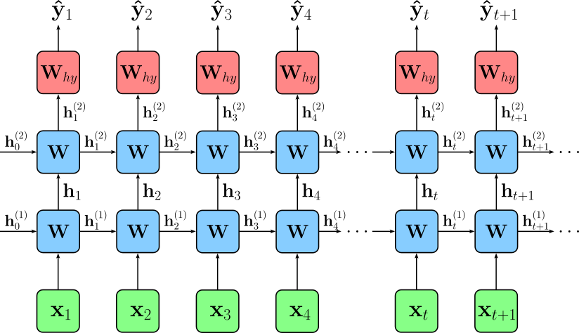
Using the default parameter of the model class (see below), we are training a 2-layer RNN. A 2-layer RNN (also called a stacked RNN) is a recurrent neural network where multiple RNN layers are placed on top of one another. The first RNN layer receives the input sequence, processes it over time, and produces a sequence of hidden states. Instead of sending these hidden states directly to an output layer, they are fed as inputs into a second RNN layer, which performs another round of temporal processing. This stacked structure allows the network to learn more complex hierarchical patterns in sequential data — lower layers may capture short-term or local patterns, while higher layers can model longer-term or more abstract dependencies. This deeper structure generally improves modeling power compared to a single-layer RNN, although it may require more computation and careful regularization. The figure below shows the overall architecture.
In this notebook, we will be using an LSTM (Long Short-Term Memory) network. This is a specialized type of RNN designed to overcome the limitations of a "vanilla RNN", particularly the problem of vanishing and exploding gradients during backpropagation through time. While a vanilla RNN uses a single hidden state that is repeatedly updated, an LSTM introduces a more complex internal structure with multiple gates — input, forget, and output gates — along with a cell state that can carry information forward over long time spans. These gates learn to regulate what information to store, update, and discard, giving LSTMs much stronger control over long-range dependencies.
The main benefit of LSTMs is their ability to remember information over significantly longer sequences compared to vanilla RNNs. This makes them far more effective for tasks such as language modeling, translation, speech recognition, and time-series forecasting. Additionally, because LSTMs reduce gradient decay, they train more stably and capture richer patterns, while still being flexible enough to forget irrelevant information through their gating mechanisms. The class LstmLM implements the complete network architecture.
class LstmLM(nn.Module):
    def __init__(self, vocab_size, embed_size=256, hidden_size=512, num_layers=2, dropout=0.2):
        super().__init__()
        self.vocab_size = vocab_size
        self.embed = nn.Embedding(vocab_size, embed_size)
        self.lstm = nn.LSTM(embed_size, hidden_size, num_layers=num_layers, batch_first=True, dropout=dropout)
        self.out = nn.Linear(hidden_size, vocab_size)
        self.num_layers = num_layers
        self.hidden_size = hidden_size

    def forward(self, x, hidden):             # x:      (batch_size, seq_len)
        emb = self.embed(x)                   # emb:    (batch_size, seq_len, embed_size)
        out, hidden = self.lstm(emb, hidden)  # out:    (batch_size, seq_len, hidden_size)
        logits = self.out(out)                # logits: (batch_size, seq_len, vocab_size)
        return logits, hidden

    def init_hidden(self, batch_size, device):
        # return tuple (h0, c0) of shape (num_layers, batch_size, hidden_dim)
        return (torch.zeros(self.num_layers, batch_size, self.hidden_size).to(device),
                torch.zeros(self.num_layers, batch_size, self.hidden_size).to(device))

    @torch.no_grad()
    def generate(self, seed_indices, eos_token=None, max_len=50, temperature=1.0, top_k=10, device='cpu'):
        seed = seed_indices.unsqueeze(0).to(device) # seed: (1, seed_seq_len)
        # Initialize hidden state with all zeros
        hidden = self.init_hidden(1, device)
        # Initialize list of generation tokens with seed tokens
        generated = seed.squeeze(0).tolist()
        # Feed the seed sequence to the model
        logits, hidden = self.forward(seed, hidden)
        # Generate remaining tokens step by step
        for _ in range(max_len):
            # Apply temperature to logits
            logits = logits[:, -1, :] / temperature
            # Top-k filtering (if specified)
            if top_k is not None and top_k < logits.size(-1):
                topk_vals, topk_idx = torch.topk(logits, top_k)
                probs = F.softmax(topk_vals, dim=-1)
                next_token = topk_idx.gather(1, torch.multinomial(probs, num_samples=1))
            else:
                # fallback to full softmax sampling
                probs = F.softmax(logits, dim=-1)
                next_token = torch.multinomial(probs, num_samples=1)
            # Stop generating tokens if the next token is the EOS token
            if eos_token is not None:
                if next_token.item() == eos_token:
                    break
            # Add new token to the final list of tokens (i.e., token indices)
            generated.append(next_token.item())
            # Pass new token and last hidden state to model
            logits, hidden = self(next_token, hidden)
        # Return final list of all tokens (seed tokens + generation tokens)
        return generated
Model Training
To train the model, we first need to instantiate the model itself, as well as the optimizer and the criterion (i.e., the loss function); just run the code cell below. Common optimizers for training RNN-based language models in PyTorch are largely the same as those used for other neural networks, but some are especially popular due to their stability and ability to handle sequential data.
The most commonly used optimizer is Adam, because it adapts the learning rate for each parameter, handles noisy gradients well, and generally converges faster than classical methods. Variants such as AdamW (Adam with decoupled weight decay) are also widely used, especially when regularization is important. Another traditional but still relevant choice is SGD with momentum, which can work well for RNNs when carefully tuned, though it often requires more manual learning-rate scheduling. Less common but still used options include RMSprop, which historically performed well on recurrent networks because it smooths gradient magnitudes over time. Overall, Adam or AdamW are the standard default optimizers for training RNN-based language models in PyTorch.
Regarding the criterion, keep in mind that the nn.CrossEntropyLoss works directly on logits because it internally applies log_softmax to convert them into log-probabilities before computing the negative log-likelihood. This design is both numerically stable and efficient: applying softmax and then taking a log would risk floating-point underflow, but combining them into a single log_softmax step avoids these issues. As a result, you can feed raw, unnormalized model outputs (logits) directly into nn.CrossEntropyLoss, and it will safely and correctly compute the cross-entropy without requiring you to apply softmax yourself.
model = LstmLM(tokenizer.vocab_size).to(DEVICE)

optimizer = torch.optim.Adam(model.parameters(), lr=1e-3)
criterion = nn.CrossEntropyLoss()

print(model)
LstmLM(
  (embed): Embedding(50257, 256)
  (lstm): LSTM(256, 512, num_layers=2, batch_first=True, dropout=0.2)
  (out): Linear(in_features=512, out_features=50257, bias=True)
)
Before we actually start with the training, let's first see how the model behaves with its randomly initialized weights. For this, we can use the generate_response() method and a simple prompt to let the model generate the next best tokens; see the code cell below.
prompt = "the best part of the movie was"

generate_response(prompt, tokenizer, model, EOS_TOKEN_INDEX)
'the best part of the movie was greatness Brut towedmd cracksggle flourishing Ame Pulse broker Ame goodkernel States padtry incapable respective incapable Casino TransportDX referral attracted rideaker happiest Continent relocation UV crou Lavrov readablebasic goddGUI pedestrians incapable incapable rib Bugsetz charitiesWelcome ISS akin sum Teslaaker Taxes'
As expected, beyond the seed words of the prompt, the output looks like a random garbled mess. However, we can use this output to compare it with one after even the first epoch.
Finally, we are ready to train the model. In the code cell below, by default, we train the model for $5$ epochs. After each epoch we either print a single generated response based on the previous example prompt (demo mode) or generate multiple example responses and save them to a file (full training mode). In the full training mode, we also save a checkpoint after each epoch.
Important: While the code below saves a checkpoint after each epoch in full training mode, it does not directly resume training after a problem by automatically loading the last checkpoint; notice that the method load_checkpoint() is actually nowhere used in the notebook. This is to keep the code as simple and clean as possible. Also, even in full training mode — and assuming a decent consumer GPU — the training time is measured in very few hours instead of days.
Also word of "warning": After only $5$ epochs, even when using all $100,000$ reviews in the full training mode, you are unlikely to see great results in terms of human-like responses. Properly training a neural network-based language model — using RNNs or Transformers — simply requires a lot of time and computational resources. We also work only with a small and domain-specific dataset that likely contains not (very) well-formed sentences. We also do not perform any kind of hyperparameter tuning in this notebook to find the best values for the embedding size, hidden size, number of layers, learning rate, etc. However, you should still be able to see how the generated responses improve over time, particularly compared to the example generated without any training (see above).
num_epochs = 5

for epoch in range(num_epochs):
    description = f"Epoch {epoch+1}/{num_epochs}"
    epoch_loss = train_epoch(loader, model, optimizer, description)
    # Generate some reponses to track progress
    if mode == "demo":
        print(generate_response(prompt, tokenizer, model, eos_token=EOS_TOKEN_INDEX))
    else:
        save_checkpoint(model, optimizer, epoch+1, epoch_loss, path=f"{folder}checkpoint-{epoch+1}.pt")
        generate_example_responses(tokenizer, model, eos_token=EOS_TOKEN_INDEX, path=f"{folder}example-responses-{epoch+1}.txt")

print(f"Done training {num_epochs} epochs.")
the best part of the movie was of.. to a of. to is the and, in the and a. in,. in the to the and the and the to is the the in to it the,,.. of to to. to to the is and to
the best part of the movie was a film for the end of the first film and a movie for a time of the first of the film was not to get it, but the first movie of the end is just to do it, the characters was a few film's film.
the best part of the movie was a bit. this is no way on this film that the film was just so bad that i had a little fan of a movie and the film was so much to see it. there is a film with the movie for a great. i don't
the best part of the movie was just as an interesting movie. i have been seen in my life. if you want for watching this. i'm not sure that you would have a good story. it would not be more better than the most annoying, but it is just plain predictable
the best part of the movie was a lot of time and that the first two of it is so much i could be disappointed with the movie with this garbage. the film is the film's "i'm sure the "gob" is an excellent movie. there wasn't the film
Done training 5 epochs.
In demo mode and after only a handful of epochs, you should be able to see the responses slowly become better, with short phrases becoming more and more coherent. However, getting the model to generate fluent and coherent response across the whole sequence requires a substantial amount of training and a sufficiently large and tuned model.
Summary
This notebook provided a clear, step-by-step walkthrough of how to train an RNN-based language model using a simple toy dataset. Rather than focusing on scale or performance, the goal was to build intuition: how to prepare sequential data, how to construct and train a recurrent model, and how to interpret its predictions. Each component, from batching to hidden-state handling, from logits to sampling, was introduced gradually so that the underlying mechanics of recurrent models become transparent rather than obscure. Along the way, we emphasized core concepts such as truncated backpropagation through time, the importance of detaching hidden states, and sequence continuation between batches. By walking through these steps in detail, the notebook demystified what is often treated as a black box, showing how an RNN maintains and updates internal state as it processes text.
Although modern large language models are almost universally based on Transformers, the ideas covered here remain highly relevant. Transformers were designed in part to overcome precisely the limitations that RNNs face, such as their difficulty capturing long-range dependencies and challenges in parallelization. Understanding where RNNs struggle gives valuable insight into why attention mechanisms, residual connections, and parallel sequence processing became so central in Transformer architectures.
At the same time, RNNs have by no means disappeared. They remain widely used in many practical domains, including speech processing, time-series forecasting, online prediction tasks, and lightweight edge models. By working through a small but complete RNN language model, this notebook highlights both the strengths and weaknesses of recurrent networks, providing intuition that helps explain the evolution of modern neural architectures — and ultimately deepens our understanding of how today's large models work under the hood.