Disclaimer: This Jupyter Notebook contains content generated with the assistance of AI. While every effort has been made to review and validate the outputs, users should independently verify critical information before relying on it. The SELENE notebook repository is constantly evolving. We recommend downloading or pulling the latest version of this notebook from Github.

Retrieval-Augmented Generation (RAG) — A (Very) Basic Example

Retrieval-Augmented Generation (RAG) is a powerful technique that enhances the capabilities of language models by grounding their responses in external, context-specific knowledge. Instead of relying solely on the model's internal parameters, a RAG pipeline retrieves relevant information from a curated dataset and feeds it to the model at generation time. This notebook provides a gentle, hands-on introduction to the core ideas behind RAG, using a very small example that highlights the essential components without the complexity of large-scale production systems.

In this notebook, we will work with a lightweight, locally-running pretrained LLM and a small dataset of news articles that serves as our knowledge repository. By keeping both the model and the dataset intentionally small, we can focus on understanding the mechanics of retrieval, the structure of the pipeline, and how the retrieved context influences the final model output. This makes it easier to experiment, visualize, and reason about what is happening at each stage.

Throughout the notebook, we will build each part of the pipeline step-by-step: preprocessing the data, creating vector embeddings, storing them in a simple index, retrieving the most relevant passages based on a user query, and finally passing this context to the LLM to produce an augmented answer. Along the way, we will explain the purpose and logic behind each stage, ensuring you gain a clear conceptual understanding of how RAG systems work.

By the end, you should have a functional minimal RAG implementation that you can run on your own machine, as well as the foundational knowledge needed to scale the approach to larger models, datasets, and more advanced architectures. This small demonstration serves as a stepping stone toward designing robust retrieval-enhanced AI applications.

Setting up the Notebook

Make Required Imports

This notebook requires the import of different Python packages but also additional Python modules that are part of the repository. If a package is missing, use your preferred package manager (e.g., conda or pip) to install it. If the code cell below runs with any errors, all required packages and modules have successfully been imported.

import numpy as np
import pandas as pd
import faiss
from transformers import AutoModelForCausalLM, AutoTokenizer
from sentence_transformers import SentenceTransformer

from src.utils.data.files import *

Download Required Data

Some code examples in this notebook use data that first need to be downloaded by running the code cell below. If this code cell throws any error, please check the configuration file config.yaml if the URL for downloading datasets is up to date and matches the one on Github. If not, simply download or pull the latest version from Github.

articles, _ = download_dataset("/text/corpora/news/sciencenews-articles-sampled.csv")

File 'data/datasets//text/corpora/news/sciencenews-articles-sampled.csv' already exists (use 'overwrite=True' to overwrite it).

Preliminaries

Before checking out this notebook, please consider the following:

• The focus of this notebook is on simplicity and clarity to understand the basic components of a RAG system and their implementation. This includes that we only consider a very small dataset for the knowledge repository and ignore considerations relevant for large-scale RAG systems (e.g., advanced chunking strategies, hybrid indexing strategies, performance considerations)

• For the generation of responses, we will be using a small, locally running, pretrained LLM instead of a Cloud-based API. The main reason is that we can be sure that the queries we will be asking cannot be answered by the LLM alone since the required information is too recent and beyond the knowledge cutoff of the model.

---

Quick Recap: Retrieval-Augmented Generation (RAG)

RAG is an approach that enhances LLM outputs by incorporating information retrieved from an external knowledge source. Instead of relying solely on what the model has learned during training — which may be incomplete, outdated, or too general — RAG dynamically fetches relevant documents, passages, or facts at query time. This makes the model's responses more grounded, accurate, and context-aware, especially in domains such as news, technical documentation, customer support, or any setting where up-to-date or specialized information is crucial. RAG can significantly reduce hallucinations, improve factuality, and enable smaller models to perform competitively by leveraging external knowledge.

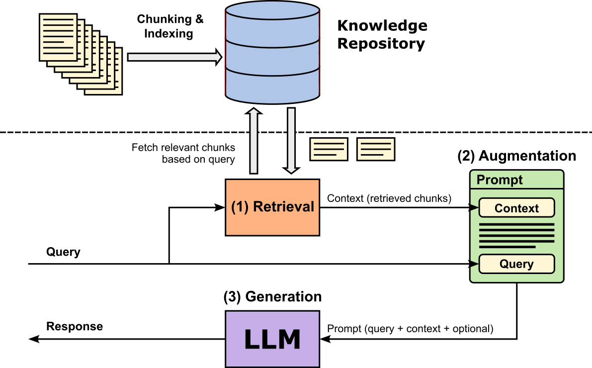
A basic RAG pipeline operates through three core steps as shown in the figure below. In the retrieval step, the system takes the user's query and uses it to find similar/related/relevant document chunks from a knowledge repository. In the augmentation step, the retrieved (and potentially ranked, filtered, etc.) chunks are combined with the original query to form an enriched prompt. This augmented input provides the LLM with external, context-specific information that it did not necessarily learn during training. Finally, in the generation step, the LLM processes this combined input and produces an answer grounded in the retrieved content. Because the model has access to relevant evidence, the output is generally more accurate, detailed, and less prone to hallucination than a standard model-only response.

In this notebook, we will create a small knowledge repository based on science news articles that were published after the pretrained model we will be using was trained. This means that we can ask questions the model, in principle, is incapable of answering correctly without having access to the relevant information. However, we will see that the model will still answer "something", and thus highlighting one of the biggest problems when using LLMs in practice: hallucinations.

---

Loading & Testing the Pretrained LLM

Instead of using a Cloud-based API to submit a prompt to an LLM, we will locally run and use a small pretrained LLM. More specifically, we will be using TinyLlama-1.1B-Chat-v1.0, a compact, instruction-tuned language model designed to offer strong conversational and reasoning capabilities at a fraction of the size of mainstream LLMs. With only 1.1 billion parameters, it is lightweight enough to run efficiently on standard CPUs or modest GPUs, making it easy to embed in small applications, notebooks, or teaching examples. Despite its small footprint, TinyLlama is trained on high-quality conversational and general-purpose data, allowing it to deliver coherent responses and follow instructions reliably.

For our simple RAG setup, the model's small size ensures fast inference while still being expressive enough to clearly demonstrate how retrieved context influences generation. More importantly, however, according to its page in Hugging Face, the model has been trained starting from Sep 1, 2023, for 90 days. This means that the training does not include any data available from 2024 onwards. We can therefore be sure that the model does not know the answer for any questions about more recent topics. This would be different if we would use a Cloud-based API to access an LLM which might search the Internet for an answer "on the fly".

The code cell below defines the model identifier TinyLlama-1.1B-Chat-v1.0 on Hugging Face. By changing the identifier to a different pretrained model, you can easily test the RAG setup using different models. By default, we use the TinyLlama model due to its small size but great performance (for its size).

model_id = "TinyLlama/TinyLlama-1.1B-Chat-v1.0"

Load Pretrained Model

To load TinyLlama-1.1B-Chat-v1.0 we can use the AutoModelForCausalLM class from the transformers library. This class automatically loads the correct causal language modeling architecture based on a model’s configuration, so you do not need to know its internal model class beforehand. By calling AutoModelForCausalLM.from_pretrained(), the library inspects the model metadata and returns an instance optimized for next-token prediction — ideal for text generation, chatbots, and RAG pipelines. Common arguments such as device_map="auto" allow Transformers to automatically distribute the model across available hardware (e.g., CPU, GPU, or multiple GPUs), while dtype="auto" selects the most efficient and compatible precision (such as float16 or bfloat16) supported by your device. These options make model loading easier, more flexible, and optimized for a wide range of hardware setups.

llm = AutoModelForCausalLM.from_pretrained(model_id, device_map="auto", dtype="auto")

Load Pretrained Tokenizer

To use a pretrained language model correctly, we also need to load the matching pretrained tokenizer because the tokenizer defines how text is converted into the model's input tokens — the exact numerical IDs the model was trained to understand. Different models use different vocabularies, special tokens, and tokenization rules, so using a mismatched or generic tokenizer can lead to incorrect token IDs, degraded performance, or even unusable output. The tokenizer ensures consistent handling of text (including punctuation, whitespace, and special formatting), and it also defines how to decode the model's outputs back into readable text. Without the correct tokenizer, the model cannot reliably interpret user input or express coherent responses, making it a critical component of any generation or RAG workflow.

tokenizer = AutoTokenizer.from_pretrained(model_id)

tokenizer.pad_token = tokenizer.eos_token

Regarding the second line in the previous code cell, setting tokenizer.pad_token = tokenizer.eos_token is often necessary because many causal language models, including Llama-style models, do not come with a dedicated padding token by default. Padding is required when batching sequences of different lengths or when using features like attention masks during generation or training. By assigning the pad_token to be the same as the eos_token, we give the model a safe, semantically neutral token that it already understands, avoiding errors or undefined behavior. This ensures that padding does not introduce unknown tokens, keeps batch processing stable, and maintains compatibility with the model's vocabulary and training setup.

Create Auxiliary Method to Prompt LLM

With the LLM and accompanying tokenizer loaded, we can now prompt the model to generate outputs. To this end the code cell below defines the method generate_output() that combines the three main required steps for a convenient use:

(1) Application of chat template. TinyLlama-1.1B-Chat-v1.0 is an instruction-tuned chat model, meaning it was trained using a specific conversation formatting style that includes system, user, and assistant roles. The tokenizer's apply_chat_template() method automatically formats a list of chat messages into the exact prompt structure the model expects such as adding role tokens, separators, and special formatting that mirrors its training data. Without applying this template, the model would receive raw text without the conversational cues it relies on, leading to inconsistent or low-quality responses.

(2) Generation of output tokens. The apply_chat_template() method not only formats the input, also also tokenizes the final prompt and converts each token to its corresponding token id or token index. The resulting sequence of token ids can now serve a valid input for the LLM to generate its response, which again is a sequence of token ids.

(3) Decoding of generated tokens. To return the response as a human-readable text, we use the tokenizer's decode() method to convert the token ids of the response back into tokens (i.e., mainly words). Lastly, We can ignore the text before the <|assistant|> tag in the model's response because everything before that tag is simply the model echoing the chat template or reconstructing the conversation context—not the actual generated answer. Since the portion before <|assistant|> is just the model repeating the prompt or template, it does not contain meaningful output; only the text after <|assistant|> represents the actual assistant-generated answer.

def generate_output(model, tokenizer, messages, max_length=100, temperature=0.01):
    # Apply prompt template and convert to token ids (important: add "<|assistant|>" as generation prompt)
    prompt_ids = tokenizer.apply_chat_template(messages, add_generation_prompt=True, return_tensors="pt").to(model.device)
    # Use model to generate output
    outputs = model.generate(
        prompt_ids,
        max_new_tokens=max_length,              # Limit the number of tokens in the response
        do_sample=True,                         # Enable sampling for diversity
        temperature=temperature,                # Sampling temperature; lower = more deterministic
    )
    # Decode the generated token IDs back into text
    response = tokenizer.decode(outputs[0], skip_special_tokens=True)
    # Extract and return only the assistant's reply (remove the prompt)
    return response.split("<|assistant|>\n")[-1].strip()

Notice the two default parameters of the generate_output() method. For one, max_length=100 limits the number of generated tokens to 100 simply to ensure that each response will not take too long to generate. By setting temperature=0.01, which is generally considered small temperature the model will produce more deterministic and conservative responses. Temperature controls how much randomness is introduced into the sampling process: lower values (close to 0) make the model favor the most probable next tokens, leading to precise, predictable, and often more factual answers. This reduces creativity and variability but increases consistency and stability, which is particularly useful for tasks like question answering, RAG pipelines, or situations where correctness is more important than diversity.

Testing the Model

We are now ready to test the pretrained LLM, first without using RAG. For this, the code cell includes two example questions referring to information not known to the model: hurricane Melissa in 2025 and the number of shark attacks in 2024. We naturally picked the question for this notebook because we know the relevant answer can be found in the documents we will be using to create the knowledge repository for our RAG system later.

Recall, that TinyLlama-1.1B-Chat-v1.0 uses a message format with system, user, and assistant roles to structure conversations, helping the model understand context and generate appropriate responses. The system role provides high-level instructions or context for the model, such as behavior guidelines or persona. The user role contains the human’s input or query, while the assistant role represents the model's generated response. We therefore need to embed the question into this required format.

query = "What were the wind speeds of hurricane Melissa?"
#query = "How many shark attacks have been in 2024 that ended deadly?"

messages = [
    {"role": "system", "content": "You are a helpful assisstant."},
    {"role": "user", "content": query},
]

# Use model to generate answer
answer = generate_output(llm, tokenizer, messages)

print(answer)

The wind speeds of Hurricane Melissa were estimated to be around 155 mph (250 km/h) on August 29, 1995, which was a Category 5 hurricane at the time.

Notice that for both question the model will not respond with "I don't know" or something similar but will generate a plausible sounding answer. However, we already mentioned that the model cannot possibly know the correct answer since the relevant information is past the model knowledge cutoff. This is one of the most basic examples of a model hallucinating: the model generates information that is plausible-sounding but factually incorrect, misleading, or entirely made up. In other words, the model produces confident responses that do not reflect reality or the underlying data it was trained on.

---

Creating the Knowledge Repository

The knowledge repository is the core component of any RAG pipeline as it serves as the external source of truth that an LLM can consult when generating answers. Its purpose is for the model to retrieve relevant documents, passages, or structured data from this repository to ground its responses in accurate, up-to-date, and domain-specific information. In practice, the repository can take many forms: a collection of text files, a vector database of embedded documents, a relational database, or even a hybrid system. Its key purpose is to store information in a way that allows efficient retrieval, typically through vector similarity search or keyword search.

Source Documents

To keep it simple, we consider a dataset of 187 news articles to create the knowledge repository. More specifically, we use articles from ScienceNews.org, a long-running, nonprofit science magazine published by the Society for Science & the Public. It provides independent, up-to-date coverage of scientific research and discoveries across diverse fields like biology, physics, health, Earth science, and technology. The dataset contains all 187 articles published in the months of August, September, and October of 2025, and therefore published after the knowledge cutoff of our pretrained LLM.

We provide the articles in a single .csv file, containing the publication date, the title, the url, and the content for all articles. The content has already been preprocessed to remove all the HTML markup. The content of the article is now a simple list of paragraphs, with paragraphs separated by two newline characters. Given this simple format, we can directly load all article into a Pandas DataFrame:

df = pd.read_csv(articles)

print(f"Number of articles: {len(df)}")

Number of articles: 187

Before going on, let's also have a brief look at the content of the DataFrame.

df.head()

	PUBLISHED	TITLE	URL	CONTENT
0	2025-10-31 12:00:00-04:00	A new AI technique may aid violent crime foren...	https://www.sciencenews.org/article/ai-violent...	Crime scene clues from blowflies may help reve...
1	2025-10-31 10:00:00-04:00	Cancer treatments may get a boost from mRNA CO...	https://www.sciencenews.org/article/cancer-imm...	The mRNA COVID-19 vaccines might make some can...
2	2025-10-30 12:36:11-04:00	Nanotyrannus was not a teenaged T. rex	https://www.sciencenews.org/article/nanotyrann...	For decades, researchers have debated whether ...
3	2025-10-30 10:00:00-04:00	This flower smells like injured ants — and fli...	https://www.sciencenews.org/article/flower-emi...	A Japanese flower lures in its pollinators wit...
4	2025-10-29 12:43:40-04:00	Some planets might home brew their own water	https://www.sciencenews.org/article/planets-ma...	Some planets might produce their own water ins...

Chunking

Recall, the knowledge repository for RAG systems typically does not store and index complete documents, but instead first splits documents into chunks which then are stored and indexed. This has several practical and performance-related reasons:

• Improved retrieval accuracy. Long documents often contain many unrelated topics, so retrieving an entire document increases the chance that irrelevant or noisy text will be fed into the LLM. Smaller, semantically coherent chunks allow the retriever to match queries to just the most relevant portions, leading to more precise grounding and reducing hallucinations.

Boost retrieval efficiency. Vector databases work best when embeddings represent focused ideas. Embedding an entire long document dilutes meaning and harms similarity scoring, while embedding short sections produces more meaningful vectors. Chunking also allows the system to retrieve only the necessary fragments, saving computation and bandwidth.

Better generation quality. LLMs have context-window limits, so feeding in an entire document wastes space and may exceed model capacity. Well-sized chunks ensure that retrieved information fits comfortably into the prompt while still providing useful detail.

As the news articles are not very long, we probably do not really need to split them into chunks. However, since our focus is to cover the main components and steps of a RAG pipeline, we do chunk the news articles. In practical RAG systems, the quality of retrieval often depends on how well documents are broken into meaningful chunks. Many existing libraries (e.g., LangChain, LlamaIndex, and Haystack) provide a variety of advanced chunking strategies, including semantic splitting, recursive character splitting, and token-aware chunking — a full exploration is beyond the scape of this notebook. These tools help automate the process and are optimized for real-world workloads, where large corpora and complex document structures benefit from sophisticated preprocessing.

However, for the purpose of this notebook, the goal is clarity and foundational understanding rather than using full-featured frameworks. Therefore, we implement a simple manual chunking approach to demonstrate the core idea in the most transparent way possible. By crafting the chunking "by hand", you can clearly observe how documents are segmented, how embeddings are generated for each chunk, and how retrieval operates over this structure, thus offering an intuitive grasp of the mechanics behind more advanced RAG pipelines.

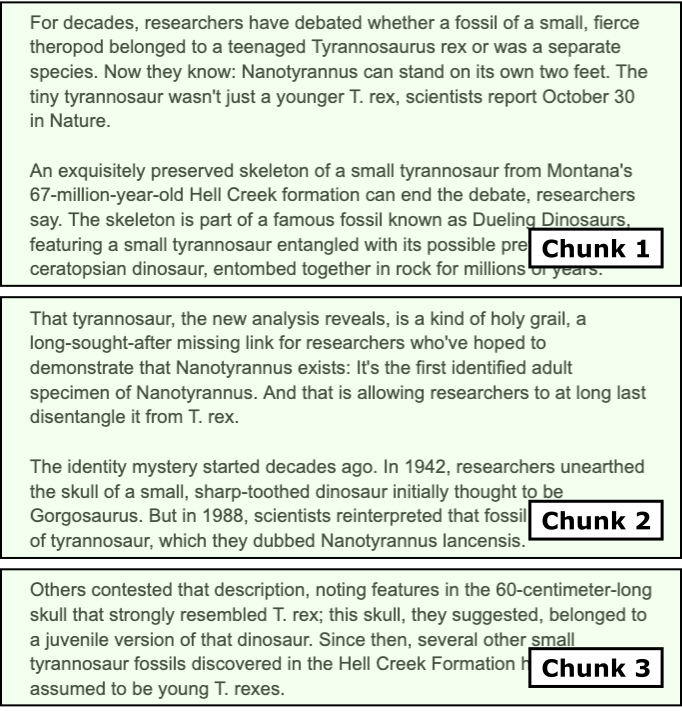
To keep it simple, we consider a simple but meaningful chunking strategy: We first split each document into a list of paragraphs. Then, iterating through all paragraphs, we combine paragraphs into a chunk as long as the length of the chunk in terms of tokens is below a specified threshold. Of course, we also want to make sure the splitting only happens between two chunks and never within a chunk. The figure below illustrates this idea, where an article is split into $3$ chunks and no chunk length exceeds the maximum length limit.

The method split_document() in the code cell below implements this task of splitting a single input document into chunks. Since we already know that paragraphs are separated by $2$ newline characters, splitting the document into a list of paragraphs is trivial. The main part of the method is to iterate over all paragraphs to check if multiple adjacent paragraphs should form a single chunk. To this end, the method keeps track of the current length of the chunk and checks if adding a new paragraph would exceed the specified limit. Notice that we need the tokenizer here since we need to know the length of a paragraph in terms of its number of tokens.

def split_document(content, tokenizer, max_tokens=200, paragraph_separator="\n\n"):
    # Split document into a list of paragraphs
    paragraphs = [ p.strip() for p in content.split(paragraph_separator) ]
    chunks, chunk, token_count = [], [], 0
    for p in paragraphs:
        # Tokenize paragraph and encode to token ids
        tokens = tokenizer.encode(p)
        # Check if we can add paragraph to current chunk        
        if token_count + len(tokens) <= max_tokens:
            # If so, add paragraph to current chunk
            chunk.append(p)
            token_count += len(tokens)
        else:
            # I not, add current chunk to final list + create new chunk from paragraph
            chunks.append("\n\n".join(chunk))
            chunk = [ tokenizer.decode(tokens[:max_tokens], skip_special_tokens=True) ]
            token_count = len(tokens[:max_tokens])
    # Add eny remaining content as its own chunk
    if token_count > 0:
        chunks.append("\n\n".join(chunk))
    return chunks

We can now iterate through all rows in our Pandas DataFrame containing all news articles and split each article into chunks. For each chunk, we not only store the text (i.e., the combined paragraphs) but also metadata such as the publication date, the title and the url of the article. We later see how this can be used to provide references/sources when generating responses and returning them to users — one of the main benefits of RAG!

Just run the code cell below to generate all chunks. Since our collection of documents is very small, this will not take long.

chunks = []

for idx, row in df.iterrows():
    published, title, url, content = row
    article_chunks = split_document(content, tokenizer)
    for chunk in article_chunks:
        chunks.append({
            "text": chunk,
            "metadata": {"published": published, "title": title, "source": url}
        })

print(f"Total number of chunks: {len(chunks)}")

Total number of chunks: 1312

We are now ready to store and index our generated chunks into a knowledge repository.

Indexing

To make use of the chunk, we not only have to store them but also make them searchable so that the retriever can effectively and efficiently find the most relevant chunks given a user's questions. There are two common approaches for indexing chunks in RAG systems, full-text search or vector search, each offering different strengths depending on the use case. Full-text search relies on keyword or term-based matching, using techniques such as inverted indexes, tokenization, and ranking algorithms like BM25. Its main advantages are speed, transparency, and precision for queries with clearly matching vocabulary. It also works very well on structured or technical text where keywords are stable and predictable. However, its biggest limitation is that it struggles with semantic similarity: if the user's query uses different wording or phrasing than the original text, full-text search may fail to retrieve relevant chunks.

Vector search, on the other hand, embeds chunks and queries into dense numerical vectors and retrieves results based on semantic similarity rather than exact keyword overlap. This allows it to capture deeper meaning, making it robust to paraphrasing, synonyms, and concept-level queries. As a trade-off, vector search is more computationally expensive, requires embedding models, and may return semantically “close” but not necessarily precise or factual matches. In practice, many RAG systems combine both approaches (often called hybrid search) to achieve both precise keyword matching and strong semantic recall.

For our practical example here, we will be using the vector search approach to benefit from semantic similarity search. However, this means that we need a model to embed chunks and queries into meaningful embedding vectors. Luckily, many pretrained models for this task exist and are publicly available. Our embedding model of choice in this notebook is all-MiniLM-L6-v2, a lightweight, high-performance sentence-embedding model from the SentenceTransformers family. It is based on a distilled version of Microsoft's MiniLM architecture and produces 384-dimensional embeddings optimized for semantic similarity, clustering, and information retrieval tasks. Despite being small and fast, it delivers strong performance across a wide range of benchmarks, making it one of the most popular embedding models for RAG systems and semantic search.

embed_model_id = "sentence-transformers/all-MiniLM-L6-v2"

To load the model, we can use the SentenceTransformer class that is part of the sentence_transformers Python library, designed to make working with sentence- and document-embedding models simple and intuitive. Under the hood, it wraps transformer-based architectures and handles tokenization, batching, and model inference, making embedding generation accessible with just a few lines of code. To load the pretrained all-MiniLM-L6-v2** model, we simply instantiate the class with the model name. The library automatically downloads the model (if not cached) and prepares it for use.

embed_model = SentenceTransformer("sentence-transformers/all-MiniLM-L6-v2")

Once loaded, we can call model.encode() on text or lists of documents to generate embeddings that can be stored in a vector index or used directly for semantic search.

To store and index the vectors for searching, we are using FAISS (Facebook AI Similarity Search), an open-source library developed by Meta AI for efficient similarity search and clustering of dense vectors. It is widely used in RAG systems, recommendation engines, and large-scale vector databases because it can store millions to billions of embeddings and retrieve the nearest neighbors extremely fast. FAISS provides both exact and approximate search algorithms and supports CPU and GPU acceleration, making it suitable for high-performance applications. The benefits of FAISS include speed, scalability, and flexibility: it handles massive datasets efficiently, offers GPU acceleration, and provides multiple indexing strategies to balance accuracy and performance. It is one of the most widely used tools for vector search in production-grade RAG pipelines.

The code cell below performs all the required steps:

• Encoding of chunks. First we convert all chunks (more specifically, the text of each chunk) into its vector representation by encoding the chunk using the pretrained all-MiniLM-L6-v2 embedding model. Since our collection of chunks is very small, we can do this for all chunks at once to get a list of embedding vectors. Notice that we set normalize_embedding=True in the encode() method,

to L2-normalize all embedding vectors (see reason below).

• Storing and indexing embedding vectors with FAISS. FAISS supports different indexing strategies. Here, we are using the IndexFlatIP to perform exact nearest-neighbor search using Inner Product (IP) as the similarity metric. "Flat" means the index stores all vectors directly without compression or hierarchical structures, so the search is exhaustive but still highly optimized in C++. Inner Product search is commonly used when embeddings are L2-normalized, because maximizing the inner product becomes equivalent to maximizing cosine similarity. For this reason, IndexFlatIP is popular in RAG systems and semantic search setups where normalized vectors make similarity comparisons more meaningful. Its advantages include simplicity, high accuracy (since it performs exact search), and strong performance for small‐to-medium-sized embedding collections. The trade-off is that it does not scale as efficiently as FAISS’s approximate indexes when working with very large datasets (e.g., hundreds of millions of vectors).

• Store metadata. FAISS only supports storing and indexing embedding vectors but not any accompanying metadata. We therefore keep all metadata in a separate Python dictionary using the chunk ids as the keys for quick access.

# Create embeddings
chunk_texts = [c["text"] for c in chunks]
chunk_embeddings = embed_model.encode(chunk_texts, convert_to_numpy=True, normalize_embeddings=True)

# Build FAISS index
dim = chunk_embeddings.shape[1]
index = faiss.IndexFlatIP(dim)
index.add(chunk_embeddings)

# Maintain side metadata mapping
metadata = {i: chunks[i]["metadata"] for i in range(len(chunks))}

Note that, by default, FAISS stores all indexes in memory, which allows for extremely fast similarity search and low-latency retrieval. This makes it ideal for real-time applications or workflows where the index fits comfortably in RAM. However, FAISS also provides methods to serialize and save an index to disk using functions like faiss.write_index() and faiss.read_index(). This enables persistent storage, sharing across systems, or reloading large indexes without recomputing embeddings, making it practical for production environments or workflows that require long-term retention of the vector database. For our small RAG system, however, we simply keep everything in memory.

---

RAG-Based Prompting

With the knowledge base created — which in practice is typically the most challenging and time-consuming part to get right — we can now implement our RAG pipeline containing the three main steps of retrieval, augmentation, and generations.

Retrieval

The FAISS index allows us to find the most relevant chunks given a user query. To show an example, in the code below, we first take the example query from the beginning, and use the embedding model to convert the query into its corresponding embedding vector. We can then use the FAISS index to find the most relevant chunks by finding the chuck embedding vectors most similar to the query embedding vector. In the example below, we return the top-2 most relevant chunks; we print chunks as well as their metadata.

query_vector = embed_model.encode([query], convert_to_numpy=True, normalize_embeddings=True)
distances, indices = index.search(query_vector, 2)
print(indices)

print("Top matches:\n")
for rank, idx in enumerate(indices[0]):
    print(f"======== Chunk {rank+1} ========")
    print(f"{chunks[idx]['text']} (score: {distances[0][rank]:.4f})\n")
    print(f"   Metadata: {metadata[idx]}")
    print()

[[60 61]]
Top matches:

======== Chunk 1 ========
With winds whirling at about 290 kilometers per hour, Hurricane Melissa is one of the strongest ever recorded in the Atlantic Ocean — and is poised to become the strongest storm ever to make landfall in Jamaica. It's also a huge storm, with hurricane-force winds extending over 70 kilometers from its core. Hours before official landfall, heavy rains and battering winds had already begun to lash the island.

After the Category 5 storm roars ashore over Jamaica on October 28, its path will take it spinning over Cuba, Haiti and the Dominican Republic. Those in its path are bracing for catastrophic flash flooding and landslides, storm surge and waves, and intense winds powerful enough to destroy homes and infrastructure. (score: 0.6465)

   Metadata: {'published': '2025-10-28 10:02:47-04:00', 'title': 'Hurricane Melissa spins into a monster storm as it bears down on Jamaica', 'source': 'https://www.sciencenews.org/article/hurricane-melissa-monster-storm-jamaica'}

======== Chunk 2 ========
The story of this latest hurricane sounds all too familiar: The slow-moving storm was initially unfocused and disorganized, but two days of lingering over deep, warm ocean water gave it enough fuel to whip itself into a tightly spinning catastrophic force of nature, centered around a piercingly sharp eye.

Such rapid intensification of tropical storms into major hurricanes has become the norm as ocean temperatures continue to rise around the globe. Climate change models have projected that hurricanes will also move more slowly as the planet warms — not only giving the storms time to gather more energy from the hot water, but also to dump copious amounts of rain after landfall. Forecasters are projecting that Melissa is holding so much moisture that it could dump as much as a meter of rain on Jamaica. (score: 0.6238)

   Metadata: {'published': '2025-10-28 10:02:47-04:00', 'title': 'Hurricane Melissa spins into a monster storm as it bears down on Jamaica', 'source': 'https://www.sciencenews.org/article/hurricane-melissa-monster-storm-jamaica'}

For a more convenient use, we can combine all steps into a method get_context() (see below), which returns the context as the concatenation of all relevant chunks as well as a set containing all the sources (i.e., the urls of the news articles the chunk came from). Since multiple chunks may be taken from the same article, we return a set of sources to remove duplicate urls.

def get_context(query, model, index, chunks, metadata, topk=2):
    # Embed query string to vector    
    query_vector = model.encode([query], convert_to_numpy=True, normalize_embeddings=True)
    # Find indices most similar check embedding vectors
    distances, indices = index.search(query_vector, topk)
    # Create context as the combination of all relevant cunks
    context = "\n\n".join([ chunks[idx]["text"] for idx in indices[0] ])
    # Extract the corresponding sources for each chunk (remove duplicates, if needed)
    sources = set([ metadata[idx]["source"] for idx in indices[0] ])
    # Return context and sources
    return context, sources

Let's run the method for the example query and inspect the result.

context, sources = get_context(query, embed_model, index, chunks, metadata)

print(f"Context and sources for query '{query}'\n")
print(context)
print(sources)

Context and sources for query 'What were the wind speeds of hurricane Melissa?'

With winds whirling at about 290 kilometers per hour, Hurricane Melissa is one of the strongest ever recorded in the Atlantic Ocean — and is poised to become the strongest storm ever to make landfall in Jamaica. It's also a huge storm, with hurricane-force winds extending over 70 kilometers from its core. Hours before official landfall, heavy rains and battering winds had already begun to lash the island.

After the Category 5 storm roars ashore over Jamaica on October 28, its path will take it spinning over Cuba, Haiti and the Dominican Republic. Those in its path are bracing for catastrophic flash flooding and landslides, storm surge and waves, and intense winds powerful enough to destroy homes and infrastructure.

The story of this latest hurricane sounds all too familiar: The slow-moving storm was initially unfocused and disorganized, but two days of lingering over deep, warm ocean water gave it enough fuel to whip itself into a tightly spinning catastrophic force of nature, centered around a piercingly sharp eye.

Such rapid intensification of tropical storms into major hurricanes has become the norm as ocean temperatures continue to rise around the globe. Climate change models have projected that hurricanes will also move more slowly as the planet warms — not only giving the storms time to gather more energy from the hot water, but also to dump copious amounts of rain after landfall. Forecasters are projecting that Melissa is holding so much moisture that it could dump as much as a meter of rain on Jamaica.
{'https://www.sciencenews.org/article/hurricane-melissa-monster-storm-jamaica'}

Augmentation

The augmentation step in a RAG pipeline refers to the process of enriching the model's input with retrieved context from the knowledge repository. The retrieved chunks are combined with the original query, often by concatenating them into a single prompt or input sequence, so that the language model can use them as context when generating a response. Since the TinyLlama-1.1B-Chat-v1.0 uses the common role-based message format, we can define a template that appropriately combines both the context and the user query, supplemented with meaningful system message.

messages = [
    {"role": "system", "content": "You are provided with the following context:"},
    {"role": "user", "content": context},
    {"role": "system", "content": "You are a helpful assisstant. Use the provided context to generate a short response. Explain how you derived the answer from the provided content"},
    {"role": "user", "content": query},
]

Keep in mind that there is not a single best way to phrase the system message, to order the context and prompt, etc. The proposed template merely follows best practices such as telling the LLM to focus on the provided context.

Generation

The last step is to simply pass the final prompt to the LLM to generate the response. As we have already defined an auxiliary method generate_output() we can just call it with the prompt containing the context and user query and inspect the returned response.

answer = generate_output(llm, tokenizer, messages)

print(answer)

The provided context states that Hurricane Melissa is one of the strongest ever recorded in the Atlantic Ocean, with winds whirling at about 290 kilometers per hour. The wind speeds of hurricane-force winds extending over 70 kilometers from its core are also mentioned. Therefore, the wind speeds of hurricane Melissa are estimated to be in the range of 290-300 kilometers per hour.

For either of the two example queries defined at the beginning of the notebook, you should now see that the response is factually correct. You can check the correctness by comparing it with the most relevant chunk used as context as these chunks stem directly from the published news articles (which, of course, we assume are correct).

Putting it all Together

With all three steps implemented, we can combine retrieval, augmentation, and generation into a single method to query our simple RAG system more easily; see the method generate_rag_ouput() below. Note that the method uses the all default parameters of the methods get_context() (the number of retrieved chunks) and generate_output() (the maximum length of the response and the temperature) to keep the code clean and simple. However, extending the method generate_rag_output() to provide these parameters as input as straightforward.

def generage_rag_output(query, embed_model, index, chunks, metadata, llm, tokenizer):
    # (1) Retrieval
    context, sources = get_context(query, embed_model, index, chunks, metadata)
    # (2) Augmentation
    messages = [
        {"role": "system", "content": "You are provided with the following context:"},
        {"role": "user", "content": context},
        {"role": "system", "content": "You are a helpful assisstant. Use the provided context to generate a short response. Explain how you derived the answer from the provided content"},
        {"role": "user", "content": query},
    ]
    # (3) Generation
    answer = generate_output(llm, tokenizer, messages)
    return answer, sources

We can now use this single function to submit user queries to our RAG pipeline.

query = "What were the wind speeds of hurricane Melissa?"
#query = "How many shark attacks have been in 2024 that ended deadly?"

answer, sources = generage_rag_output(query, embed_model, index, chunks, metadata, llm, tokenizer)

print(f"Query: '{query}'\n")
print(f"Answer:\n{answer}")
print(f"Sources: {sources}")

Query: 'What were the wind speeds of hurricane Melissa?'

Answer:
The provided context states that Hurricane Melissa is one of the strongest ever recorded in the Atlantic Ocean, with winds whirling at about 290 kilometers per hour. The wind speeds of hurricane-force winds extending over 70 kilometers from its core are also mentioned. Therefore, the wind speeds of hurricane Melissa are estimated to be in the range of 290-300 kilometers per hour.
Sources: {'https://www.sciencenews.org/article/hurricane-melissa-monster-storm-jamaica'}

Important: Although our basic implementation of a RAG pipeline seems to work well, it is important to highlight a critical limitation of this solution. Recall that the get_context() method returns the, by default, $2$ most relevant chunks for a given user query. However, since we did not specify any minimum similarity, we will always get $2$ chunks even for queries that do not match any meaningful chunk. To show this, we can submit queries that the pretrained LLM can answer without any context from the knowledge base; see the code cell below.

query = "What is the capital of France?"
#query = "What are the main ingredients of bread?"

answer, sources = generage_rag_output(query, embed_model, index, chunks, metadata, llm, tokenizer)

print(f"Query: '{query}'\n")
print(f"Answer:\n{answer}")
print(f"Sources: {sources}")

Query: 'What is the capital of France?'

Answer:
The capital of France is Paris.
Sources: {'https://www.sciencenews.org/article/nasas-webb-telescope-moon-uranus', 'https://www.sciencenews.org/article/coral-collapse-climate-tipping-point'}

Notice that the LLM may still provide the correct answer by "ignoring" the provided context. However, this might not always be the case for all kinds of queries. As indicated above, one way to address this is to define a miniumum similiarity between the query vector and chunk vectors, and dismiss and chunk below this threshold. Since the search() method of FAISS returns both the indices of the most relevant chunks as well as the distances/similarities, filtering out chucks with an insufficient similarity is trivial.

However finding a meaningful similarity threshold in practice can be tricky because embedding scores are not inherently standardized across queries or datasets. The numerical range of cosine similarity or inner product depends on factors such as the embedding model, vector normalization, and the dimensionality of embeddings. A score that indicates a strong semantic match in one context might be weak in another, making it difficult to choose a single threshold that reliably separates relevant from irrelevant chunks across all queries.

Additionally, different queries have different "semantic density". Some queries are very specific, making even moderate similarity scores meaningful, while others are broad, where only very high similarity scores indicate true relevance. This variability means that a fixed threshold can either exclude useful information or include noisy, irrelevant chunks. As a result, practitioners often experiment with thresholds empirically, adjust them dynamically based on query characteristics, or rely on ranking and top-k strategies combined with thresholds to balance recall and precision. These considerations, although very important in practice, go beyond the scope of this introductory notebook.

---

Discussion

The RAG pipeline we implemented and showcased in this notebook, using a small example dataset, represents the most basic RAG implementation since the focus here was in simplicity and clarity. Building effective and efficient RAG pipelines for real-world application is much more challenging. While the three main steps of retrieval, augmentation, and generation still form the backbone, their implementation requires more careful considerations. In the following, we briefly outline some of the potentially added complexity.

• Advanced chunking strategies. Our dataset of news articles was very well-behaved in a sense that documents were simply a list of (typically short) paragraphs. In real-world RAG systems, documents often have complex structures that go beyond simple continuous text. Articles, reports, or technical manuals may include tables, bullet points, code snippets, or even conversational transcripts. If these documents are naively split, chunks may cut across logical boundaries, separating related information or combining unrelated pieces. To handle such complexity, more advanced chunking strategies are often required. Semantic or structure-aware chunking can detect natural boundaries such as table rows, bullet points, or dialogue turns, ensuring each chunk represents a coherent concept. Recursive or hierarchical splitting approaches can preserve context in long documents while maintaining manageable chunk sizes for embedding.

• Multimodal content. Instead of just text content — like used here in this notebook — documents for RAG systems may be multimodal, containing not only text but also images, charts, diagrams, or other visual elements. These non-textual components often carry critical information that cannot be captured through text embeddings alone. Ignoring these elements can lead to incomplete or misleading context being provided to the language model, reducing the quality and accuracy of generated responses. Incorporating multimodal content affects the implementation of a RAG pipeline in several ways. First, it requires additional preprocessing steps, such as extracting image features using computer vision models or converting charts into structured data representations. Second, embeddings must be generated for both textual and visual content, and retrieval mechanisms must be able to handle these heterogeneous embeddings in a coherent way. Finally, the augmentation step must integrate multimodal information effectively, ensuring that the language model can reason over text and visual evidence simultaneously. This adds complexity to the pipeline but is essential for building RAG systems that can leverage the full richness of modern documents.

• Vector search vs. full text-search. In this notebook, we considered vector search to support the semantic retrieval of chunks. While vector search is powerful for capturing semantic similarity, it can sometimes introduce challenges in RAG systems. One issue is that embeddings may retrieve chunks that are semantically related but factually incorrect or only loosely relevant to the query. For example, two concepts might be contextually similar in embedding space but differ in critical details, leading the language model to hallucinate or provide misleading answers. Additionally, vector search performance and relevance depend heavily on the quality of the embedding model and the choice of similarity metric, which may not generalize well across all queries or domains. In cases where exact keyword matches or precise terminology are important, a full-text search or a hybrid approach may be preferable. Full-text search excels at retrieving documents containing specific terms, numbers, or named entities, which is crucial in technical, legal, or scientific texts. Hybrid approaches combine the strengths of both vector and keyword-based search, first narrowing candidates using keywords and then ranking them semantically. This ensures both precision and semantic relevance, reducing the risk of retrieving irrelevant or misleading chunks while still benefiting from the flexibility of vector-based similarity.

• Scaling & efficiency. Since we used only a small pretrained model and a very small dataset, performance was not a concern for our basic RAG pipeline. Building an efficient RAG pipeline at large scale, with millions of documents, introduces several significant challenges. Firstly, storage and retrieval efficiency becomes critical, as embedding millions of chunks can require hundreds of gigabytes of memory or disk space. Simple in-memory indexes may no longer be feasible, and even vector search algorithms can become computationally expensive if not optimized. Efficient indexing structures, approximate nearest-neighbor search, and distributed storage solutions are often necessary to keep latency low while maintaining acceptable retrieval quality. And secondly, updating and maintaining the knowledge repository becomes more complex at scale. Adding new documents, reindexing embeddings, and ensuring consistency across distributed systems can be time-consuming and error-prone. Additionally, managing retrieval quality across diverse document types and domains is harder, since embeddings and chunking strategies may vary in effectiveness. Large-scale systems also need to balance precision, recall, and latency, often requiring hybrid search, caching, and prioritization strategies to ensure the RAG pipeline remains practical and responsive in real-world applications.

---

Summary

This Jupyter notebook provided a practical introduction to building a Retrieval-Augmented Generation (RAG) system using a locally running pretrained language model and a small dataset of news articles. The goal was to illustrate the fundamental components of a RAG pipeline, including document chunking, embedding generation, vector storage and retrieval using FAISS, and augmentation of the query with retrieved information for grounded text generation. By walking through each step with simplified, "by-hand" implementations, the notebook made the inner workings of RAG systems transparent and accessible for educational purposes.

The notebook demonstrated how to break documents into chunks to improve retrieval relevance, encode each chunk into vector embeddings using the all-MiniLM-L6-v2 model, and store these embeddings in a FAISS index. It showed how retrieval works by finding the most semantically similar chunks for a given query and how these retrieved chunks are then augmented with the user query to provide context for the language model. This simple example highlights the interplay between retrieval and generation, which is the key insight behind RAG: the model no longer relies solely on its parametric memory but can access external, up-to-date information.

While this notebook focused on clarity and simplicity, it is important to note that real-world RAG systems involve many additional considerations. These include handling very large datasets, ensuring efficient and scalable indexing, dealing with memory and latency constraints, dynamically selecting relevant chunks, and managing information freshness. Other practical concerns, such as multi-modal data, hybrid retrieval strategies combining vector and keyword search, and safety or guardrails to reduce hallucinations, were deliberately left out to keep the example understandable.

Overall, the notebook served as a hands-on educational tool to explore the mechanics of RAG without the complexity of production-scale implementations. By implementing each step manually, you can develop a stronger intuition about how retrieval, augmentation, and generation interact and why each component matters. This foundational understanding is essential for anyone aiming to build more advanced or production-ready RAG systems in the future.