Disclaimer: This Jupyter Notebook contains content generated with the assistance of AI. While every effort has been made to review and validate the outputs, users should independently verify critical information before relying on it. The SELENE notebook repository is constantly evolving. We recommend downloading or pulling the latest version of this notebook from Github.

Time Series Analysis — An Overview

Time series analysis is concerned with the study of data that are observed sequentially over time. Unlike cross-sectional data, where observations are typically assumed to be independent, time series often exhibit temporal dependencies, trends, seasonal effects, structural changes, and other dynamic patterns. Understanding these temporal relationships is essential for extracting meaningful information from data and for supporting informed decision-making across a wide range of domains.

Time series analysis plays a central role in numerous real-world applications. In healthcare, it is used to monitor patients' vital signs and detect early indicators of disease. In economics and finance, it supports the analysis of economic indicators, stock prices, and unemployment rates. In manufacturing and engineering, sensor measurements are continuously analyzed to detect faults and predict equipment failures, while in retail and energy systems, historical demand is used to optimize inventory management and resource planning. These diverse applications illustrate that time series analysis extends far beyond forecasting and encompasses tasks such as understanding historical behavior, monitoring evolving systems, and anticipating future developments.

This notebook provides a high-level overview of the field of time series analysis. It introduces common application areas involving temporal data, discusses the main types and characteristics of time series, and presents an overview of widely used methods and models for their analysis. Rather than focusing on implementation details or mathematical derivations, the notebook aims to develop an intuitive understanding of the concepts that underlie modern time series analysis.

The objective is not to provide an exhaustive treatment of every topic, but instead to establish a solid foundation for further study. By the end of this notebook, you should be familiar with the fundamental terminology, recognize common properties of time series data, understand the objectives of different analysis tasks, and gain an overview of the basic approaches that form the basis of more advanced time series methods.

Setting up the Notebook

This notebook does not contain any code, so there is no need to import any libraries.

---

Introduction

Motivation

Time series data consist of observations collected sequentially over time, where the temporal order of the observations carries essential information about the underlying process. Unlike cross-sectional data, individual observations are generally not independent, but instead exhibit temporal dependencies, trends, seasonal patterns, and other dynamic behaviors. Time series arise naturally in a wide range of scientific and industrial applications, including financial markets, healthcare, manufacturing, environmental monitoring, transportation, and energy systems, making their analysis fundamental for understanding complex temporal phenomena and supporting data-driven decision-making.

Example 1. Continuous monitoring of a patient's vital signs is one of the most prominent applications of time series analysis in healthcare. Measurements such as heart rate, blood pressure, respiratory rate, blood oxygen saturation, and electrocardiograms are recorded sequentially over time, allowing clinicians to assess a patient's current condition, detect early signs of deterioration, and anticipate adverse events. The ability to analyze these temporal patterns is therefore essential for supporting timely diagnosis, clinical decision-making, and patient care. For example, the plot below shows the recorded heart beats for a patient across $12$ seconds.

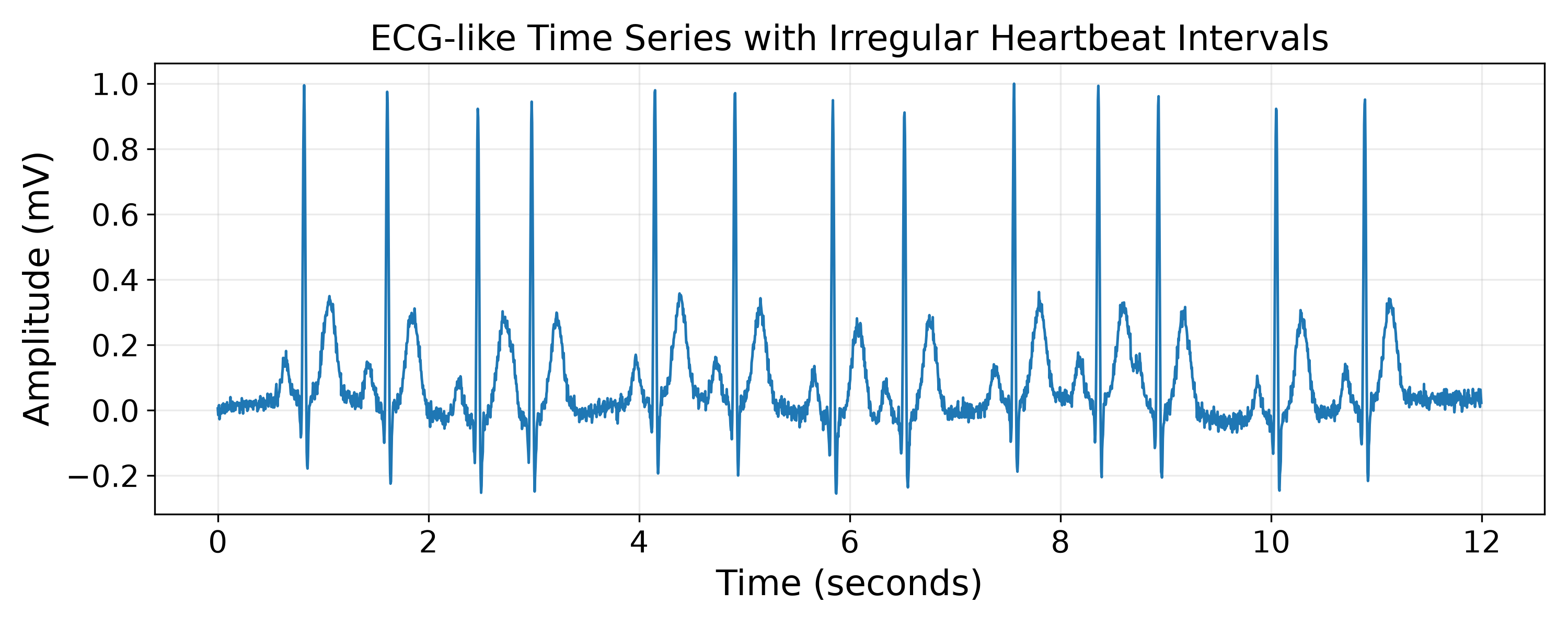
The heartbeat is irregular because the intervals between successive peaks vary substantially: some beats occur unusually early, while others are followed by longer pauses. In a healthy resting rhythm, these intervals are typically more consistent, so pronounced variability may suggest abnormal electrical activity such as ectopic beats or an arrhythmia. However, a person's heart rate depends on their current physical activity and other factors, so simply using a fixed threshold to indicate a "normal" distance between peaks does not work. We therefore need more sophisticated methods to detect irregular heartbeats.

Example 2. Analyzing a product’s sales over time (such as daily units sold) is a common application of time series analysis in economics and business. Sales data often exhibit temporal patterns caused by seasonality, weekends, holidays, promotions, price changes, and broader economic conditions. Identifying and forecasting these patterns helps firms understand consumer demand, plan inventory and staffing, evaluate marketing activities, and make better production and pricing decisions. The example plot below shows the daily sales of a product over a single year, showing a clear peak during the summer months.

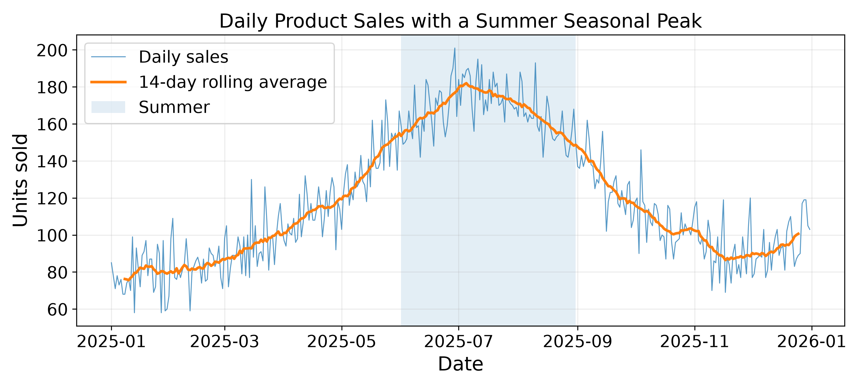
Insights gained from sales time series can directly support operational and strategic business decisions. By identifying recurring demand patterns and anticipating periods of high or low sales, companies can optimize inventory levels, reduce the risk of stockouts or excess inventory, and improve supply chain planning. At the same time, sales trends can inform pricing strategies, guide the timing and targeting of advertising campaigns, and help evaluate or schedule promotional activities to maximize customer engagement and revenue. As a result, time series analysis enables businesses to make proactive, data-driven decisions that improve both operational efficiency and commercial performance.

Example 3. Analyzing a country's unemployment rate over time is a fundamental application of time series analysis in economics. Changes in unemployment reflect the combined effects of economic growth, labor market conditions, government policies, and external events, providing valuable insights into the overall health of an economy. The plot below shows the unemployment rate for a country across a year. In this example, we highlight a sudden change — typically referred to as a structural break — where the unemployment rate suddenly increases.

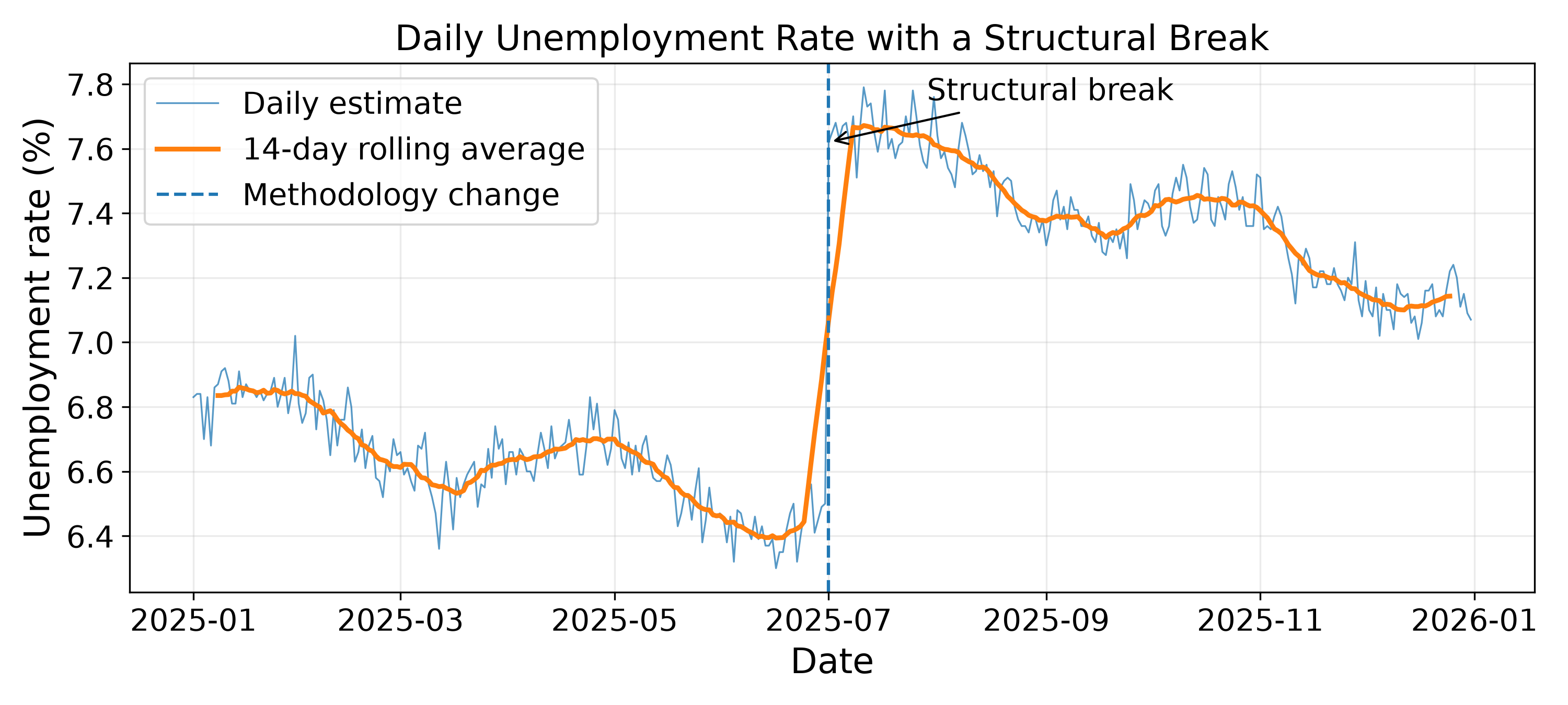
By identifying long-term trends, seasonal fluctuations, and structural breaks, policymakers and economists can evaluate the impact of economic measures, monitor labor market dynamics, and make informed decisions on fiscal, monetary, and employment policies. For example, a structural break as shown in the plot above might indicate the effect of a major policy change or simply a change in the methodology of how the unemployment rate is calculated.

In short, time series analysis is widely used across domains such as healthcare, economics, finance, manufacturing, transportation, and environmental science because many real-world processes evolve over time. At the same time, temporal data and the associated analytical tasks can take many forms: series may be regular or irregular, univariate or multivariate, short or long, and may contain trends, seasonality, anomalies, or structural breaks. Accordingly, time series analysis encompasses a broad range of objectives, from understanding historical patterns and monitoring current conditions to forecasting future developments and supporting practical decisions.

To provoide a comprehensive overview to different tasks, to different types and characteristics of time series, as well as to common methods and models is the purpose of this notebook.

Basic Definitions

In its most fundamental form, a time series $\mathcal{S}$ is mathematically most commonly defined as an ordered sequence of observations indexed by time, which we can express as

$$\large \mathcal{S} = \{x_t\}_{t \in \mathcal{T}}, $$

where $\mathcal{T}$ is the time index set (e.g., ${1,\ldots,T}$, but also $\mathbb{N}$ or $\mathbb{R})$; and $x_t \in \mathcal{X}$ is the observation at time $t$. For a finite discrete time series, which we typically work with in practice, we can express a times series as tuple of observations:

$$\large \mathbf{x} = (x_1, x_2, \ldots, x_T) $$

For example, the time series below shows the hourly observations of a patient's heart rate across $5$ hours.

$$\large \mathbf{x} = (72, 75, 74, 78, 76) $$

As a limitation, this notation assumes that all observations have been collected or sampled at regular time intervals (e.g., every hour for our example recording a patient's heart rate). While this is a common situation in practice — and many models assume regularly sampled observations — this is not a fundamental requirement of a times series. For example, a time series tracking the patient's urine volume over many days is unlikely to be observed in regular time intervals.

In this case, we need to extend the previous definition to explicitly the time stamp of an observation. As a result, a single observation is now a tuple containing both the time stamp and the values, giving us:

$$\large \mathcal{S} = \{(t_i, x_i)\}_{i=1}^{T} $$

For the patient example, the first tuple $(t_1, x_1)$ might look like $(\text{"2025-01-01 08:00"}, 72)$. Of course, we still assume hourly recorded observations here, the second tuple $(t_2, x_2)$ would be $(\text{"2025-01-01 09:00"}, 75)$, and so on. This example also shows why we do not need to explicitly denote the time stamp $t_i$ if we have regularly sampled data.

Our current definition of a time series assumes that we are recording only a single observation (e.g., a patient's heart rate). However, a time series might record multiple vital signs (e.g., heart rate, body temperature, blood pressure) at the same time. We can express this by denoting all observations at a time stamp as vector $\mathbf{x}_i$ (instead of a scalar value $x_i$):

$$\large \mathcal{S} = \{(t_i, \mathbf{x}_i)\}_{i=1}^{T} $$

Lastly, we might want to record and analyze the vital signs of multiple patients together. This means that we also have to explicitly specify the patient — or more generally, the entity, subject, or instance. To denote the time series for the $n$-th entity $e^{(n)}$, we therefore write:

$$\large \mathcal{S}^{n} = \{(e^{(n)}, t^{(n)}_i, \mathbf{x}^{(n)}_i)\}_{i=1}^{T_n} $$

For example, $e^{(n)}$ may be the patient ID, $t^{(n)}_i$ the hourly time stamps since admission, and $\mathbf{x}^{(n)}_i$ the collection of vitals signs.

With that, the complete dataset of time series for all $N$ entities is then simply defined as:

$$\large \mathcal{D} = \{\mathcal{S}^{(n)}\}_{n=1}^{N}, $$

In practice, we typically only use the definition we "need". For example, we consider only the time series for a single patient, which records several vital signs at regular time intervals, the definition $\large \mathcal{S} = \{\mathbf{x}_t\}_{t \in \mathcal{T}}$ is sufficient and appropriate.

Side note: The distinction between one or more entities, as well as between one or more recorded observations at each time stamp, refers to the notion of dimensionality of a time series dataset, which we discuss in more detail when covering important types and characteristics of time series later on.

Important: The notation used for time series observations varies across the literature. Classical textbooks on statistics, econometrics, and state-space models often denote observations by $y_t$, reserving $x_t$ for latent states or explanatory variables. In contrast, contemporary machine learning literature commonly uses $x_t$ to represent observed data, particularly when time series are treated as sequences of input vectors — and then use, say, $z_t$ to denote latent states. These choices are purely notational and have no mathematical implications, provided they are used consistently. Throughout this notebook, we adopt the notation $x_t$ for observations, as it aligns with modern machine learning conventions and naturally extends to multivariate time series.

---

Common Tasks & Applications

Different ways to look at time series data for different reasons. Depending on the application, you may seek to extract meaningful patterns from historical observations, monitor evolving systems as new data arrive, or anticipate future behavior to support planning and decision-making. These objectives require different analytical techniques and address complementary aspects of temporal data.

In this section, we provide an overview of the diverse tasks involved in time series analysis by organizing them into three broad categories: understanding the past, which focuses on uncovering historical patterns and structures; real-time monitoring, which emphasizes the detection of changes and anomalies as data are observed; and predicting the future, which aims to forecast upcoming values and trends.

Looking Back: Understanding the Past

When we analyze a time series to "understand the past" our goal is generally descriptive and explanatory rather than predictive — although any insights may later help to make predictions, if applicable. The objective is to characterize the historical behavior of a process, identify the mechanisms that generated the observations, and extract knowledge that can support scientific understanding or later decision-making. The table below outlines the most common descriptive and explanatory tasks together with practical examples:

Task	Goal	Typical insights	Example applications
Exploratory analysis	Summarize the temporal behavior	Trends, seasonality, variability, outliers	Understanding electricity demand over several years
Pattern discovery	Identify recurring structures	Daily, weekly, yearly cycles; recurring motifs	Human activity recognition, ECG signals
Trend estimation	Estimate long-term evolution	Growth, decline, structural evolution	Population growth, climate change
Seasonality analysis	Quantify periodic effects	Magnitude and timing of seasonal cycles	Retail sales peaks during holidays
Change-point detection	Find historical regime shifts	Policy changes, equipment replacement, market transitions	Detecting when a machine began degrading
Anomaly analysis	Explain unusual observations	Rare failures, fraud, sensor malfunctions	Investigating unexpected network traffic
Segmentation	Partition the series into homogeneous intervals	Different operating regimes	Driving phases, sleep stages
Similarity search & motif discovery	Find repeated or similar subsequences	Frequently occurring behaviors	Repeated machine cycles
Time series clustering	Group similar time series	Common behavioral patterns	Customer energy consumption profiles
Representation learning / feature extraction	Learn compact descriptions	Latent dynamics, embeddings	Downstream classification or retrieval
Causal and intervention analysis	Understand why behavior changed	Effect of events or interventions	Impact of marketing campaigns or new policies

In other words, the insights produced by these tasks typically answer questions such as

• "What happened?"
• "How did it happen?"
• "When did it change?"
• "Why might it have happened?"
• "How similar is this behavior to previous observations?"

As you can see, even the seemingly narrow objective of "understanding the past" encompasses a diverse set of time series analysis tasks. Rather than merely summarizing historical observations, these tasks aim to uncover the underlying structure and dynamics of temporal data by identifying trends, seasonal patterns, recurring motifs, regime changes, anomalies, and relationships between observations.

Real Time: Monitoring the Present

The second perspective of time series analysis is "understanding the present", often referred to as real-time monitoring or online analysis. Here, the objective is no longer to explain historical behavior but to continuously assess the current state of a system as new observations arrive. The emphasis is on timely detection, diagnosis, and response rather than retrospective analysis or long-term prediction; common tasks and examples include:

Task	Goal	Typical insight	Example applications
Online anomaly detection	Detect unusual observations as they occur	Is the system behaving abnormally right now?	Network intrusion detection, fraud detection
Change-point detection (online)	Detect regime changes immediately	Has the process fundamentally changed?	Equipment degradation, market shifts
Fault detection & diagnosis	Identify failures and determine their cause	Which component is malfunctioning?	Industrial process monitoring
Health monitoring	Estimate the current condition of a system	Is the machine/patient operating normally?	Predictive maintenance, ICU monitoring
State estimation	Infer hidden system states	What is the current operating mode?	Robotics, autonomous vehicles, navigation
Activity recognition	Classify the current behavior	What is the person doing now?	Wearables, smart homes
Event detection	Detect occurrences of specific events	Has an earthquake/seizure/failure occurred?	Seismology, medicine
Threshold monitoring	Trigger alerts when limits are exceeded	Is a safety constraint violated?	Temperature, pressure, financial risk
Quality monitoring (SPC)	Monitor manufacturing processes	Is production still in control?	Statistical process control
Streaming classification	Continuously classify incoming sequences	Which class best describes the current signal?	Human activity, speech recognition

Compared with historical analysis (i.e., "understanding the past"), the emphasis of real-time monitoring is on situational situational awareness and timely intervention; typically trying to answer questions such as:

• "What is happening now?"
• "Has something (just) changed?"
• "Should immediate action be taken?" (e.g., an alert triggered)
• "What caused the alert?"

Real-time monitoring poses unique challenges because decisions must be made continuously as data arrive, often under strict latency and computational constraints. Unlike offline analysis, future observations are unavailable, requiring algorithms to operate incrementally while remaining robust to noise, missing data, and evolving data distributions (concept drift). Moreover, practical monitoring systems must balance the timely detection of critical events with minimizing false alarms, as inaccurate or delayed decisions can lead to substantial operational, financial, or safety-related consequences.

Looking Ahead: Predicting the Future

The third major perspective of time series analysis is "predicting the future", where the objective is to estimate future behavior based on historical observations. Unlike descriptive analysis or real-time monitoring, predictive tasks aim to support planning and decision-making under uncertainty by forecasting future values, events, or system states. Depending on the application, predictions may range from a few milliseconds ahead to years into the future. Such applications include:

Task	Goal	Typical insight	Example applications
Time series forecasting	Predict future values	What will the signal look like?	Electricity demand, stock prices, weather
Multi-step forecasting	Predict a sequence of future observations	How will the system evolve over the next hours/days?	Energy load, traffic forecasting
Probabilistic forecasting	Quantify prediction uncertainty	How likely are different future outcomes?	Renewable energy generation, finance
Remaining Useful Life (RUL) prediction	Estimate time until failure	When will maintenance be required?	Predictive maintenance
Early event prediction	Predict events before they occur	Will a failure, seizure, or attack happen soon?	Healthcare, cybersecurity
Risk prediction	Estimate the probability of adverse outcomes	How likely is a critical event?	Financial risk, patient deterioration
Trajectory prediction	Predict future paths or movements	Where will the object move next?	Autonomous driving, aircraft tracking
Demand prediction	Forecast future resource needs	How much demand should be expected?	Retail inventory, cloud computing
Scenario forecasting	Predict outcomes under different assumptions	How will the system evolve under different conditions?	Climate projections, economics

Unlike historical or real-time analysis, the primary output is not an explanation of current behavior but an estimate of future outcomes together with their associated uncertainty. Thus, predictive analysis addresses mainly questions such as:

• "What is likely to happen next?"
• "When will something happen?"
• "How certain is the prediction?"
• "What decisions should be made?"

Predicting the future is often closely tied to acting on the future. Forecasts, risk estimates, or early event predictions are rarely ends in themselves; instead, they provide the basis for decisions such as scheduling maintenance, allocating resources, adjusting production, or issuing warnings before critical events occur. In this sense, predictive time series analysis naturally extends to decision support and proactive planning.

More generally, however, all aspects of time series analysis ultimately aim to enable informed decision-making. Understanding the past provides insights that guide strategic planning and scientific discovery, real-time monitoring supports timely interventions and operational control, and predicting the future enables proactive actions under uncertainty. While these perspectives differ in their temporal focus and analytical objectives, they all transform temporal data into actionable knowledge that informs decisions in practical applications.

---

Types and Characteristics of Time Series Data

Time series occur in many different forms and exhibit a wide range of characteristics that reflect the nature of the underlying process and the way the data are observed. For example, a time series may contain trends or seasonal patterns, consist of regular or irregular observations, be univariate or multivariate, or exhibit changing statistical properties over time. These characteristics determine how the data should be interpreted and analyzed.

Understanding and identifying the characteristics of a time series is an important first step in any time series analysis. Different statistical, machine learning, and deep learning models rely on different assumptions and are designed to capture specific types of temporal behavior. Selecting an appropriate modeling approach therefore requires an understanding of the properties of the data. The following sections provide a structured overview of the core characteristics commonly encountered in time series and discuss their implications for analysis and forecasting.

While there are different ways to organize those characteristics, we favor a structure aligns naturally with the decisions you are likely to make when first exploring a new time series dataset:

• How is the data organized? $\Rightarrow$ Observation Structure + Dimensionality
• What patterns does it contain? $\Rightarrow$ Temporal Structure
• Can I assume the process is stable? $\Rightarrow$ Statistical Properties
• What practical issues must I handle? $\Rightarrow$ Data Quality & Complexity

This progression mirrors a typical time series workflow: understand the data collection, inspect temporal patterns, assess statistical assumptions, and finally address practical complications before selecting an appropriate model. It also creates a clear bridge to the next chapter on model selection, since each group of characteristics motivates a different family of methods.

Observation Structure

The observation structure of a time series describes how the data are collected and recorded over time. It characterizes the measurement process rather than the underlying temporal behavior of the series. Important aspects include whether observations are recorded at regular or irregular time intervals, the sampling frequency (e.g., hourly, daily, or monthly), whether the underlying process is observed in discrete or continuous time, and the presence of missing observations or measurement noise.

Regularity

Regularity refers to whether observations in a time series are recorded at consistent time intervals. A regularly sampled time series has a fixed sampling frequency, such as hourly temperature measurements, daily stock closing prices, or monthly sales figures, whereas an irregularly sampled time series contains observations separated by varying time intervals, such as financial transactions, patient visits, or equipment failures. Regularity is an important characteristic because many classical time series models assume equally spaced observations and rely on fixed temporal lags.

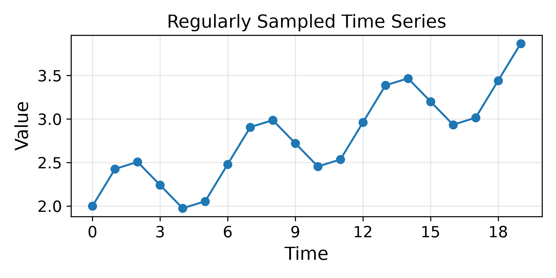
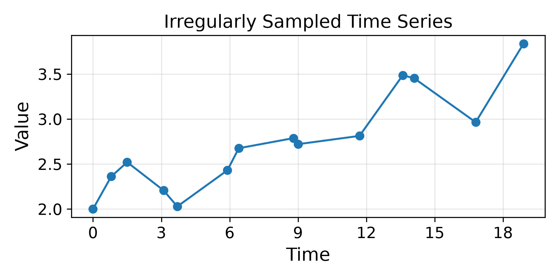
To give an example, the two plots below show a regularly sampled and an irregularly sampled time series while keeping the underlying signal nearly identical, i.e., both time series observe the same phenomenon, only at different time steps. Notice how the overall "look" of both plots is quite different — at least when using a line plot in case we assume that we can interpolate values between observed time steps.

Side note: In general, models that can handle irregularly sampled data can also be applied to regularly sampled data. After all, regular sampling is simply a special case where the time interval between successive observations is constant.

Slightly irregularly sampled time series can often be converted into regularly sampled data through preprocessing techniques such as resampling, interpolation, or aggregation. This is generally appropriate when the sampling intervals deviate only moderately from the desired frequency, the underlying process changes smoothly between observations, and no important events are lost during resampling. For example, hourly sensor measurements with occasional missing timestamps can often be interpolated onto a regular hourly grid, while irregular transaction data may be aggregated into daily totals. However, when observations are highly irregular, event-driven, or contain long gaps, resampling may distort the temporal dynamics or introduce artificial information. In such cases, models that explicitly account for irregular sampling are generally more appropriate than forcing the data onto a regular time grid.

Sampling Frequency

The sampling frequency of a time series specifies how often observations are recorded, such as every millisecond, second, hour, day, or month. It determines the temporal resolution of the data and influences which patterns can be observed and modeled. High-frequency data capture rapid changes but are often larger and noisier, whereas low-frequency data provide a coarser view of long-term behavior. The sampling frequency also affects model selection, feature engineering, and preprocessing, since different forecasting methods and temporal patterns are appropriate at different time scales. The table below shows some common examples.

Sampling Frequency	Typical Example	Typical Application
Milliseconds to microseconds	Stock trades	High-frequency finance
Seconds	ECG or wearable sensor readings	Healthcare monitoring
Minutes	Traffic flow measurements	Intelligent transportation systems
Hourly	Electricity demand	Energy forecasting
Daily	Hospital admissions	Healthcare operations
Weekly	Retail sales	Business analytics
Monthly	Unemployment rate	Economic analysis
Quarterly	Gross Domestic Product (GDP)	Macroeconomics
Yearly	Population size	Demographic studies

Time Domain

The time domain of a time series describes whether the underlying process is defined at discrete points in time or continuously over time. A discrete-time series consists of observations recorded at specific time steps, such as hourly temperatures, daily stock closing prices, or monthly sales, and is the setting assumed by most classical time series models. In contrast, a continuous-time process is defined for every instant in time, such as a patient's heart rate, the position of a moving vehicle, or the temperature of a chemical reactor.

In practice, however, truly continuous observations are rarely available because measurements are collected by digital sensors or recording systems at finite sampling frequencies. As a result, most real-world datasets are discrete-time observations of an underlying continuous-time process. The distinction is nevertheless important because it influences both the choice of models and the interpretation of the data, particularly when observations are irregularly sampled or the sampling frequency is low relative to the dynamics of the underlying process.

Missing Data

Missing values occur when one or more observations in a time series are unavailable at their expected time points. They are a common data quality issue that can disrupt temporal dependencies and affect the performance of forecasting and analysis methods, particularly those that assume complete and regularly sampled data. Here are some common causes:

Cause	Description	Example
Sensor failure	Measurement device temporarily stops recording data.	Missing temperature readings due to a malfunctioning weather station.
Communication failure	Data are lost during transmission or storage.	Missing IoT sensor readings caused by a network outage.
Equipment maintenance	Measurements are intentionally suspended during servicing.	Production sensors turned off during scheduled maintenance.
Human factors	Observations are missed due to manual recording errors or skipped measurements.	A patient misses a scheduled medical examination.
Market or operational closures	No observations are collected because the system is inactive.	No stock prices on weekends or public holidays.
Data corruption	Observations are removed because they are invalid or unreadable.	Corrupted telemetry records discarded during data cleaning.
Sampling limitations	Some observations are intentionally omitted due to cost or resource constraints.	Environmental samples collected only every second day instead of daily.

Depending on the cause and extent of the missing values, they may be handled through interpolation, imputation, or by using models that explicitly accommodate incomplete observations.

Measurement Noise

Measurement noise refers to random or systematic errors introduced during the observation process that cause recorded values to differ from the true underlying signal. Unlike the natural variability of the process itself, measurement noise arises from imperfections in sensors, instruments, or data collection procedures; for example:

Cause	Description	Example
Sensor precision limits	Instruments have finite measurement accuracy and resolution.	Small fluctuations in digital temperature sensor readings.
Electronic interference	Electrical noise affects sensor signals or communication channels.	Noise in ECG or EEG recordings caused by nearby electrical devices.
Environmental influences	External conditions interfere with measurements.	Wind affecting weather station measurements or dust affecting optical sensors.
Calibration errors	Sensors become biased due to incorrect or outdated calibration.	A pressure sensor consistently overestimates the true pressure.
Quantization	Continuous signals are rounded to discrete digital values during analog-to-digital conversion.	A smart meter reports electricity consumption only to the nearest 0.1 kWh.
Human measurement error	Manual observations introduce random or systematic inaccuracies.	Slight differences in blood pressure measurements taken by different clinicians.
Data acquisition artifacts	Noise is introduced during recording, transmission, or preprocessing.	Compression artifacts or signal distortion in wireless sensor networks.

Excessive measurement noise can obscure temporal patterns, reduce forecasting accuracy, and complicate the identification of trends, seasonality, or anomalies. Depending on its magnitude and characteristics, measurement noise may be reduced through filtering, smoothing, calibration, or models that explicitly account for observation uncertainty.

Structural Breaks

A structural break is abrupt and lasting changes in the statistical properties of a time series, such as its mean, variance, trend, or seasonal pattern; recall the example plot showing the unemployment rate of a country above. Unlike temporary fluctuations or recurring regimes (see below), structural breaks typically result from permanent changes in the underlying data-generating process, such as policy interventions, technological innovations, or major external events.

Application	Typical Structural Break	Example
Economic indicators	Policy or regulatory change	Inflation behavior changes after a new monetary policy.
Retail sales	Permanent shift in consumer behavior	Online shopping permanently increases after the COVID-19 pandemic.
Manufacturing	Equipment replacement	Machine vibration characteristics change after installing a new production line.
Energy consumption	Infrastructure or technology change	Household electricity demand decreases after widespread adoption of LED lighting.
Environmental monitoring	Climate or land-use change	River flow patterns shift following the construction of a dam.
Financial markets	Major economic event	Stock market volatility permanently increases after a financial crisis.

Ignoring structural breaks can lead to inaccurate models and forecasts because relationships learned from historical data may no longer hold after the break. Consequently, structural break detection and model adaptation are often important components of time series analysis.

Dimensionality

The dimensionality of a time series addresses two core questions

• "How many variables are observed for a single process?" — univariate vs. multivariate
• "Howm many processes are observed? — single vs. multiple processes

This fundamental distinction allows us to derive for main types of time series.

(Single) Univariate Time Series

In this most basic form of a time series, we observe only a single variable $x_t$ for a single process at each time step $t$. To give an example, the table below shows the snippet of the hourly recordings of a (single!) patient's heart rate in beats per minute (bpm).

Timestamp	Heart Rate (bpm)
2025-01-01 08:00	72
2025-01-01 09:00	75
2025-01-01 10:00	74
2025-01-01 11:00	78
2025-01-01 12:00	76

(Single) Multivariate Time Series

Here, instead of a single variable, several variables of a single process are observed simultaneously. Thus, at a time step $t$, we observe vector of values:

$$\large \mathbf{x}_t = \begin{bmatrix} x_{1,t}\\ x_{1,t}\\ \vdots\\ x_{m,t}\\ \end{bmatrix} $$

where $x_{i,t}$ is the $i$-th variable (i.e., the variable for the $i$-th process) at time step $t$. As illustration, the table below extends the previous patient example by adding additional vitals (body temperature, blood pressure).

Timestamp	Heart Rate (bpm)	Body Temperature (°C)	Blood Pressure (mmHg)
2025-01-01 08:00	72	36.8	118/76
2025-01-01 09:00	75	36.9	120/78
2025-01-01 10:00	74	37.0	119/77
2025-01-01 11:00	78	37.1	122/79
2025-01-01 12:00	76	36.9	121/78

The primary objective of multivariate time series analysis is to model not only the temporal evolution of each variable but also the interactions and dependencies between multiple variables observed over time. In the patient monitoring example, pulse, body temperature, and blood pressure each exhibit their own temporal patterns, but they are also physiologically related. For instance, an increase in body temperature due to a fever may be accompanied by an elevated pulse rate, while changes in blood pressure can influence heart rate through the body's regulatory mechanisms. By modeling these relationships jointly, multivariate time series models can exploit information shared across variables, leading to a better understanding of the underlying process and often improving forecasting, anomaly detection, and state estimation compared to modeling each variable independently.

Multiple Univariate Time Series (Panel Time Series)

Again, we record a vector of variables $\mathbf{x}_t$ at each time step $t$. However, here, each variable comes from a process with its own univariate time series. For example, the table below records the daily bed occupancy for $3$ different hospitals (again, each hospital has its own univariate time series).

Date	Hospital A	Hospital B	Hospital C
2025-01-01	184	133	97
2025-01-02	187	130	101
2025-01-03	190	134	99
2025-01-04	188	136	103
2025-01-05	192	139	105

It is important to note that panel time series do not assume independence between the processes. For example, the number of occupied beds in Hospital A might have increased from $184$ to $187$ because those three patients have been moved from Hospital B to Hospital A. The dimensionality of a time series (here: panel time series) describes only the structure of the data. Whether any dependencies are modeled depends on the chosen analysis approach and model.

Multiple Multivariate Time Series

Lastly, a time series may observe multiple variables for multiple processes. This means that we now record a vector $\mathbf{x}_{i,t}$ of variables for each process $i$ at time stamp $t$. Assuming we observe $p$ variables for each process, we can define this vector as:

$$\large \mathbf{x}_{i,t} = \begin{bmatrix} x_{i,t}^{(1)}\\ x_{i,t}^{(2)}\\ \vdots\\ x_{i,t}^{(p)} \end{bmatrix} $$

The table below shows an extension of our dataset recording the vitals for a single patient to include the vitals of multiple patients, thus yielding multiple multivariate time series.

Patient	Timestamp	Heart Rate (bpm)	Body Temperature (°C)	Blood Pressure (mmHg)
P1	2025-01-01 08:00	72	36.8	118/76
P1	2025-01-01 09:00	75	36.9	120/78
P1	2025-01-01 10:00	74	37.0	119/77
P1	2025-01-01 11:00	78	37.1	122/79
P1	2025-01-01 12:00	76	36.9	121/78
P2	2025-01-01 08:00	81	38.0	129/83
P2	2025-01-01 09:00	84	38.2	131/84
P2	2025-01-01 10:00	83	38.1	130/82
P2	2025-01-01 11:00	85	38.3	132/85
P2	2025-01-01 12:00	82	38.0	128/81
P3	2025-01-01 08:00	68	36.6	114/72
P3	2025-01-01 09:00	69	36.7	115/73
P3	2025-01-01 10:00	70	36.8	116/74
P3	2025-01-01 11:00	69	36.7	115/72
P3	2025-01-01 12:00	71	36.8	117/73

Again, the observations may or may not be independent. For example, the vitals may be dependent between patients because all patients have been admitted at the same time as the victims of an accident (e.g., food poisoning or viral infection).

Hierarchical Structure

Beyond the four main types of time series, practical time series may also be hierarchical. Here, the time series consists of observations that are organized into multiple levels of aggregation, where higher-level series are obtained by summing or aggregating lower-level series. The same process is therefore observed at different levels of detail, and the values at each level are logically related. Hierarchical time series are common in business, economics, and energy systems, where forecasts may be required both for individual entities and for aggregated groups. For example, a retail sales times series may exhibit the following hierarchy:

Hierarchy Level	Time Series
Company	Total company sales
Region	Sales in North, South, East, and West regions
Store	Sales for each individual store
Product	Sales of individual products within each store

Here, the daily sales of all products are summed to obtain each store's daily sales, store sales are aggregated into regional sales, and regional sales are further aggregated into the company's total daily sales. This hierarchical structure enables analysis and forecasting at multiple levels while preserving the relationships between them.

A hierarchical time series dataset is typically stored in long (tidy) format, where each row represents one observation for a particular entity at a particular level of the hierarchy and point in time. The hierarchy is encoded using one or more identifier columns. For the retail sales example, the dataset could look as follows:

Date	Level	Region	Store	Product	Daily Sales
2026-01-01	Company	–	–	–	1,350
2026-01-01	Region	North	–	–	700
2026-01-01	Region	South	–	–	650
2026-01-01	Store	North	N1	–	400
2026-01-01	Store	North	N2	–	300
2026-01-01	Store	South	S1	–	350
2026-01-01	Store	South	S2	–	300
2026-01-01	Product	North	N1	Bread	150
2026-01-01	Product	North	N1	Milk	250
2026-01-01	Product	North	N2	Bread	120
2026-01-01	Product	North	N2	Milk	180
2026-01-01	Product	South	S1	Bread	140
2026-01-01	Product	South	S1	Milk	210
2026-01-01	Product	South	S2	Bread	130
2026-01-01	Product	South	S2	Milk	170

The aggregation relationships are:

• Store level: N1 = Bread (150) + Milk (250) = 400
• Region level: North = N1 (400) + N2 (300) = 700
• Company level: Company = North (700) + South (650) = 1,350

This long format is commonly used because it naturally accommodates multiple hierarchical levels and scales well to large datasets. Alternatively, the information may be stored across different files.

Temporal Structure

The temporal structure of a time series describes the systematic patterns and relationships that govern how the series evolves over time. These patterns include temporal dependence between observations, long-term trends, recurring seasonality, long(er)-term cycles, and the way these components combine (e.g., additively or multiplicatively).

Temporal Dependence

Temporal dependence is what distinguishes time series analysis from conventional machine learning on tabular data: the past contains information about the present and future, and successful time series models are designed to capture and exploit these temporal relationships. However, temporal dependence is not a single feature but can take several forms, mainly:

Form of Temporal Dependence	Brief Explanation	Examples
Short-term dependence	Recent observations have the strongest influence on future values, while the dependence weakens as the time lag increases.	Daily temperature, electricity demand.
Long-range dependence	Observations remain correlated even over long time intervals, indicating persistent temporal relationships.	Internet traffic, river flow measurements.
Seasonal dependence	Observations are correlated with values one or more seasonal periods earlier, reflecting recurring patterns.	Daily temperatures across years, monthly retail sales.
Nonlinear dependence	Future values depend on past observations through nonlinear relationships that cannot be adequately captured by linear models.	Financial markets, chaotic dynamical systems.

Temporal dependence is commonly explored using tools such as lag plots, the autocorrelation function (ACF), and the partial autocorrelation function (PACF), which help identify how strongly current observations are related to previous ones.

Trends

A trend is the long-term direction or systematic change in a time series, reflecting a gradual increase, decrease, or other persistent evolution in the level of the data over time. In real-world time series, trends come in very different forms; the table below provides a brief overview including examples.

Type of Trend	Brief Explanation	Examples
Linear Trend	The series exhibits a steady increase or decrease at an approximately constant rate over time.	Population growth over a short period; gradual increase in average annual temperatures.
Nonlinear Trend	The long-term movement changes at a non-constant rate, resulting in curved or irregular growth or decline.	Technology adoption following an S-shaped curve; biological growth processes.
Exponential Trend	The rate of change is proportional to the current level, causing accelerating growth or decay.	Compound investment growth; early-stage spread of an epidemic.
Piecewise (Segmented) Trend	The trend consists of multiple linear or nonlinear segments separated by structural breaks or change points.	Sales before and after a major marketing campaign; energy consumption following a policy change.
Deterministic Trend	The trend is described by a fixed, predictable function of time (e.g., linear or polynomial), with random fluctuations around it.	Steadily increasing production output; polynomial trend in long-term climate measurements.
Stochastic Trend	The trend evolves due to accumulated random shocks rather than a fixed deterministic function, so future values depend on both time and randomness.	Stock prices modeled as a random walk; exchange rates.

The plot below shows a simple example of a time series exhibitting a linear trend.

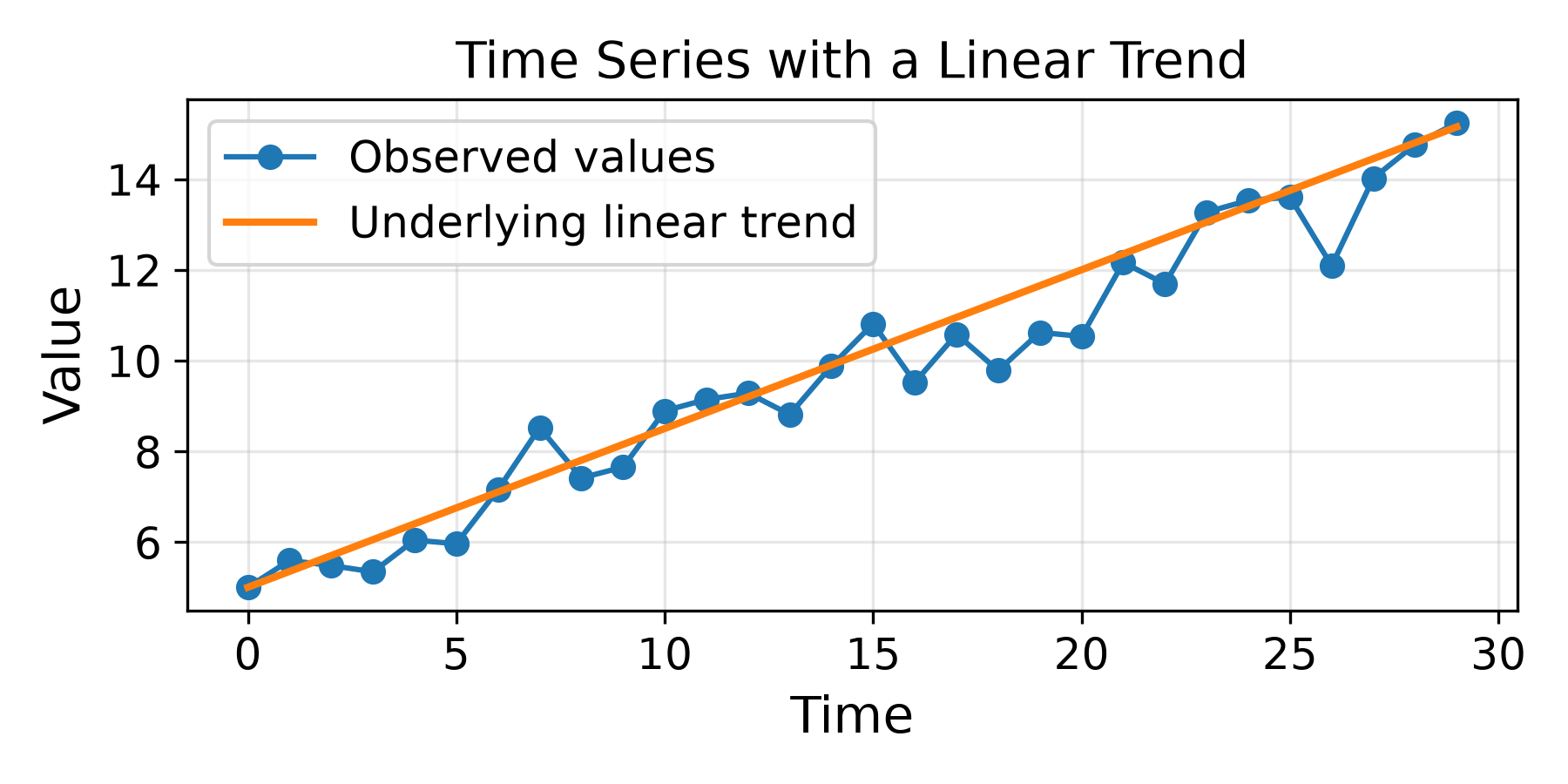
Because a trend causes the mean of the series to change over time, it generally violates the assumption of stationarity (see below), which requires the statistical properties of the series (particularly its mean and variance) to remain approximately constant. Consequently, many classical statistical models require the trend to be removed (e.g., through detrending or differencing) or modeled explicitly before the remaining stationary component can be analyzed.

Seasonality

Seasonality refers to recurring patterns in a time series that repeat at regular and predictable intervals, such as hourly, daily, weekly, monthly, or yearly cycles. These patterns are typically driven by calendar effects, environmental factors, or recurring human behavior — for example, higher electricity demand during weekdays, increased retail sales during holidays, or annual temperature cycles. Unlike a long-term trend, seasonality repeats with a fixed period and similar shape over time. Identifying and modeling seasonality is important because it explains systematic variation in the data and often improves forecasting accuracy. Some classical time series models explicitly account for seasonal patterns, while machine learning models typically capture seasonality through engineered calendar features or learned temporal representations.

Seasonality Type	Characteristics
No Seasonality	No recurring periodic pattern.
Single Fixed Seasonality	One stable seasonal period (e.g., daily, weekly, yearly).
Multiple Seasonality	Several recurring periods simultaneously (e.g., daily and weekly).
Complex or Changing Seasonality	Seasonal pattern changes in magnitude or shape over time.
Calendar Effects	Seasonal behavior tied to holidays or calendar events rather than a fixed cycle.

The time series for the daily sales of a product in the motivating example at the beginning showed that the product clearly sold better during the summer months. In terms of the different types of seasonality, this time series exhibits a single fixed seasonality (here: yearly).

Cycles

A cycle is a long-term oscillation in a time series characterized by alternating periods of growth and decline, but unlike seasonality, the timing and duration of these fluctuations are not fixed or strictly periodic. Cycles are often driven by complex underlying processes, such as economic expansions and recessions, climate phenomena, or population dynamics, and may vary in both length and amplitude. The table below highlights the main differences between seasonality and cycles.

Seasonality	Cycles
Fixed and known period	Variable and often unknown period
Calendar-driven	Process-driven
Predictable timing	Irregular timing
Examples: weekdays, months, years	Examples: business cycles, climate oscillations

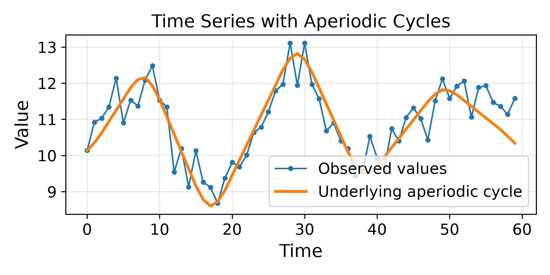
Similarly, whereas a trend describes the overall long-term direction of a series (e.g., a persistent increase or decrease), a cycle represents temporary deviations around that long-term trend. Consequently, a time series may exhibit an upward trend while simultaneously undergoing cyclical fluctuations, such as a steadily growing economy experiencing recurring business cycles. As an example, the plot below shows a simple time series containing aperiodic cycles.

Additive vs. Multiplicative

Many real-world time series can be viewed as the combination of three fundamental components:

• a trend $T_t$,
• a seasonal component $S_t$
• a residual (or irregular) component $R_t$

The trend captures the long-term direction of the series, the seasonal component represents recurring patterns that repeat over fixed intervals, and the residual accounts for random fluctuations or unexplained variation that remain after the systematic effects have been removed. This decomposition provides a useful conceptual framework for understanding the structure of a time series and motivates many classical forecasting methods, which explicitly estimate and model these components separately before combining them to describe or predict the observed data.

However, there are two main ways how this decomposition can be modeled. Firstly, the additive model assumes that the observed value of a time series is the sum of its underlying trend, seasonality, and residual. It is appropriate when the magnitude of the seasonal fluctuations remains approximately constant over time, regardless of the overall level of the series. Mathematically, an additive time series is represented as:

$$\large X_t = T_t + S_t + R_t $$

For example, the average daily temperature in a city may exhibit a gradual warming trend over several decades while maintaining a similar annual seasonal variation of roughly $\pm 10^\circ\text{C}$ each year. Since the seasonal amplitude remains approximately constant, an additive model provides a suitable representation of the time series.

Alternatively, the multiplicative model assumes that the observed value of a time series is the product of its underlying trend, seasonality, and residual**. It is appropriate when the magnitude of the seasonal fluctuations changes in proportion to the overall level of the series, so that seasonal effects become larger as the series grows. Mathematically, a multiplicative time series is represented as

$$\large X_t = T_t \times S_t \times R_t $$

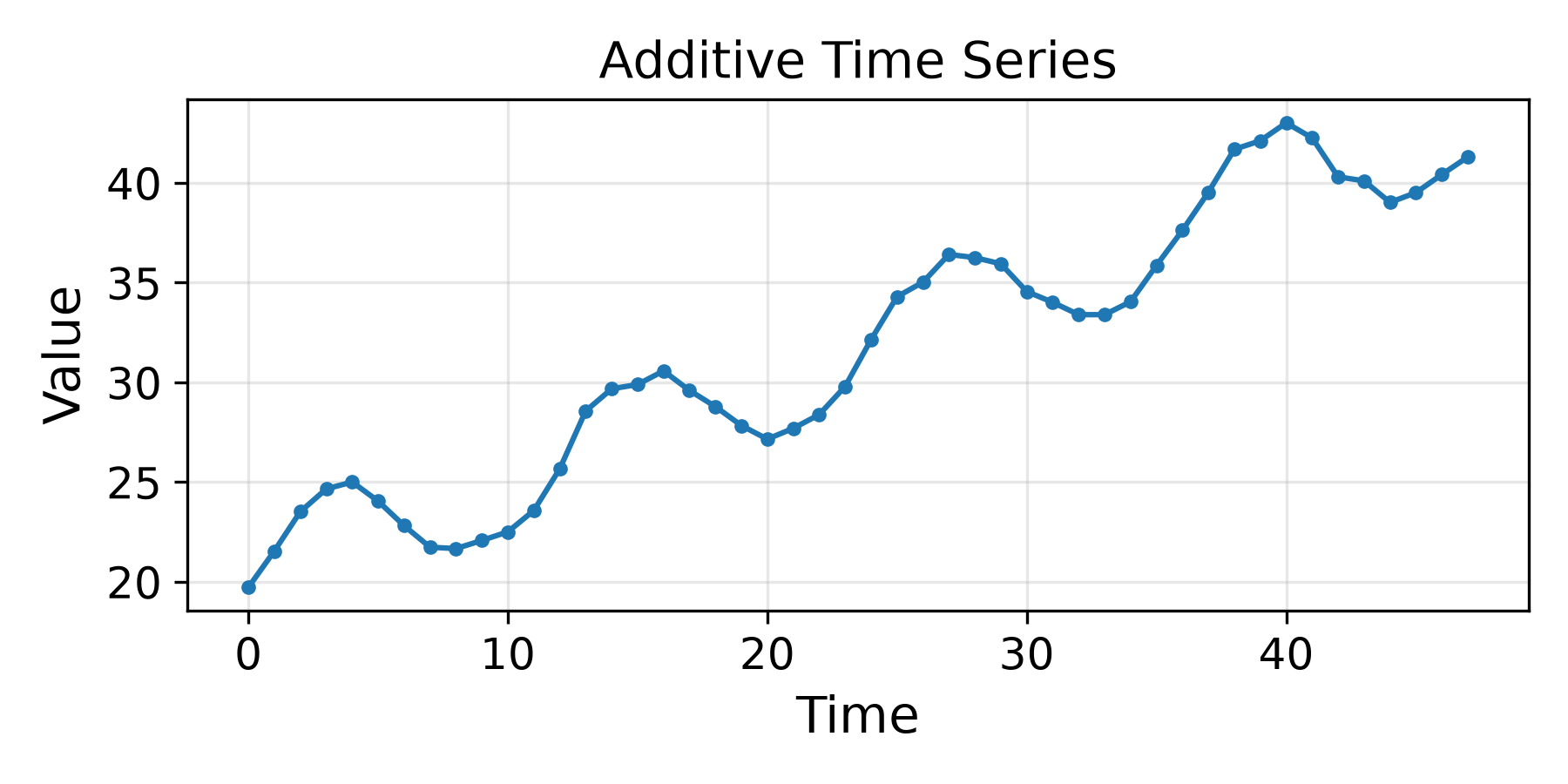
The plots below illustrate the difference between additive and multiplicative time series. In the additive series (top), the seasonal fluctuations have approximately constant amplitude regardless of the trend level. In contrast, in the multiplicative series (bottom), the seasonal fluctuations increase in amplitude as the trend increases, which is characteristic of multiplicative seasonality.

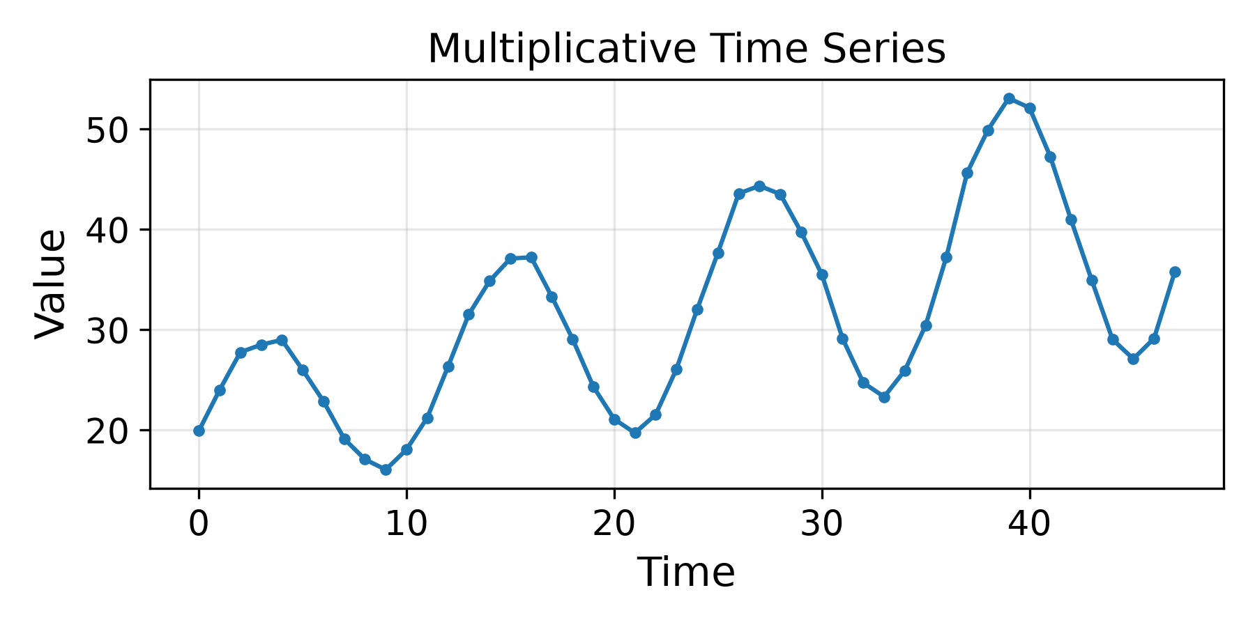
A useful property of multiplicative time series is that they can often be transformed into an additive form by applying a logarithmic transformation. Using the identity $\log{ab} = \log{a}+\log{b}$, the multiplicative model becomes:

$$\large \log{X_t} = \log{T_t} + \log{S_t} + \log{R_t} $$

This transformation converts multiplicative relationships into additive ones, making it possible to apply decomposition techniques and classical time series models that assume additive components. In practice, the logarithmic transformation is a common preprocessing step for positive-valued time series whose variability increases with their level. After fitting and forecasting on the transformed scale, the predictions are typically converted back to the original scale using the exponential function, allowing the results to be interpreted in the original units.

Statistical Properties

The statistical properties of a time series describe how its values are distributed and how these distributions evolve over time. Understanding these properties is fundamental because they determine whether assumptions such as a constant mean or variance are appropriate and influence the choice of analysis and forecasting methods. Consequently, examining the statistical properties of a time series is often one of the first steps in understanding its underlying behavior and selecting suitable models.

Stationarity

Stationarity describes whether the statistical properties of a time series remain stable over time. In a stationary series, characteristics such as the mean, variance, and temporal dependence are approximately constant, so patterns observed in the past are expected to remain relevant in the future.

Strong Stationarity. A time series is strongly (or strictly) stationary if the joint probability distribution of any collection of observations remains unchanged under shifts in time. In other words, for any set of time points $t_1, \ldots, t_n$ and any time shift $h$, the random vectors.

$$\large (X_{t_1}, \ldots, X_{t_n}) \quad\text{and}\quad (X_{t_1+h}, \ldots, X_{t_n+h}) $$

have the same probability distribution. Consequently, not only the mean and variance but all statistical properties, including higher-order moments and the complete dependence structure, are invariant over time.

Strong stationarity is a mathematically convenient concept but is rarely observed in real-world time series. Most practical data exhibit trends, seasonality, changing variability, structural breaks, or evolving dependence patterns that violate this assumption. For this reason, strong stationarity is mainly of theoretical interest, while weaker notions of stationarity are more commonly assumed in statistical time series modeling.

Weak Stationarity. A time series is weakly (or second-order) stationary if its first and second moments remain constant over time. Specifically, the process has (1) a constant mean, $E[X_t] = \mu$, (2) a constant finite variance, $\mathrm{Var}(X_t) = \sigma^2$, and (3) an autocovariance that depends only on the time lag between observations, not on their absolute position in time. That is,

$$\large \mathrm{Cov}(X_t, X_{t+h}) = \gamma(h) $$

where $\gamma(h)$ is a function only of the lag $h$. Intuitively, this means that the relationship between two observations depends only on how far apart they are in time, not on when they occur. For example, if the autocovariance at a lag of one day is high, then observations one day apart are equally related whether they occur in January, June, or December. Similarly, the relationship between observations one week apart remains the same throughout the entire time series. In a weakly stationary process, temporal dependence is therefore time-invariant: only the separation (lag) between observations matters, while their absolute position in time does not.

Unlike strong stationarity, weak stationarity does not require the entire probability distribution to remain unchanged over time, making it a less restrictive and more practical assumption. Consequently, weak stationarity is the form of stationarity most commonly assumed by classical statistical time series models.

Many real-world time series are not weakly stationary in their original form, but they can often be transformed into approximately stationary series. Depending on the source of the non-stationarity, this may involve removing a deterministic trend, differencing the series to eliminate stochastic trends, or restricting the analysis to shorter time intervals where the statistical properties remain approximately constant.

Type	Idea	Typical Transformation	Example
Trend stationary	A deterministic trend causes the mean to change over time.	Remove the estimated trend (detrending).	Long-term increase in annual average temperature.
Difference stationary	The series contains a stochastic trend (unit root).	Compute first or higher-order differences.	Stock prices or exchange rates.
Locally stationary	Statistical properties evolve slowly over time.	Analyze short time windows or use time-varying models.	EEG recordings, traffic flow, or weather measurements with changing dynamics.
Regime-switching	The series alternates between distinct operating states.	Detect regimes or use regime-switching models.	Electricity demand on weekdays versus weekends or financial markets during bull and bear periods.
Structural break	Permanent changes occur in the underlying process.	Detect break points and model segments separately or use adaptive models.	Sales before and after the introduction of a new product or policy change.

The appropriate transformation depends on the underlying cause of the non-stationarity and the assumptions of the intended analysis or forecasting model; note that we cover the notion of regimes and structural breaks in a bit more detail below.

Variance Stability

Variance stability describes whether the variability of a time series remains approximately constant over time. A time series has stable variance if the magnitude of its fluctuations does not systematically increase or decrease as time progresses. In many real-world series, however, the variance changes with the level of the series or across different time periods, a phenomenon known as heteroscedasticity. Variance stability is an important assumption for many classical statistical models, and when it is violated, transformations may be required.

Variance stability, i.e., $\mathrm{Var}(X_t)=\sigma^2$, is one of the defining conditions of weak stationarity (see above), but it alone is not sufficient. While every weakly stationary process has stable variance, a process with stable variance is not necessarily weakly stationary. For example, a time series with a strong upward trend may have constant variance but a changing mean, violating weak stationarity. Likewise, a process may have constant mean and variance but changing temporal dependence, which also violates weak stationarity.

Distribution

The distribution of a time series describes the probability distribution of its observations or, more commonly, its model residuals or innovations. Many classical statistical models assume that these quantities follow a Gaussian (normal) distribution — that is, $X_t \sim \mathcal{N}(\mu,\sigma^2)$ — which simplifies parameter estimation, statistical inference, and the construction of prediction intervals. However, real-world time series often exhibit non-Gaussian behavior, such as skewness, heavy tails, or discrete-valued observations (e.g., counts or binary events); here are a few examples:

Distribution	Typical Time Series	Reason
Approximately Gaussian	Daily average temperature	Fluctuations around the seasonal trend are often close to normally distributed.
Approximately Gaussian	Sensor measurement errors	Measurement noise is frequently modeled as Gaussian due to many small independent disturbances.
Approximately Gaussian	River water level (after detrending/seasonal adjustment)	Residual fluctuations are often symmetric and approximately normal.
Non-Gaussian (Count)	Daily emergency calls	Integer-valued counts are often modeled using Poisson or Negative Binomial distributions.
Non-Gaussian (Binary)	Machine failure indicator	Observations are binary (failure/no failure) and follow a Bernoulli distribution.
Non-Gaussian (Heavy-tailed)	Financial returns	Returns often exhibit heavy tails and extreme events that occur more frequently than predicted by a Gaussian distribution.
Non-Gaussian (Positive & Skewed)	Daily rainfall amounts	Rainfall is non-negative, highly skewed, and often includes many zero observations.
Non-Gaussian (Intermittent)	Spare parts demand	Long sequences of zeros with occasional positive values produce highly skewed, intermittent distributions.

Recognizing the underlying distribution is therefore important for selecting appropriate models, likelihood functions, and inference procedures, particularly when the Gaussian assumption is violated.

Regimes

A regime refers to a distinct operating state of a time series in which the underlying statistical behavior changes, and a single time series may feature $2$ or more regimes. Each regime is characterized by its own properties, such as mean, variance, trend, or temporal dependence, and the series switches between these states either occasionally or repeatedly. Here are some common practical examples of time series with different regimes:

Application	Typical Regimes	Example
Financial markets	Bull market, bear market, high-volatility periods	Stock returns alternate between stable growth and market downturns.
Electricity demand	Weekday vs. weekend, holiday periods	Consumption patterns differ between working days and weekends.
Traffic flow	Free-flow, congested, rush hour	Traffic speed changes between normal and rush-hour conditions.
Manufacturing	Normal operation, startup, shutdown, maintenance	Machine sensor readings differ across operating modes.
Climate and weather	Dry season, rainy season	River flow and precipitation exhibit different seasonal regimes.
Human activity	Sleep, work, exercise	Wearable sensor measurements vary across daily activity states.

The plot below shows an example of a time series with two aperiodic regimes. Such a behavior may be observed when, say, measuring a CPU temperature in a laptop when. In this case, Regime 1 might refer to the time the laptop runs on battery and therefore reduced the CPU speed; Regime 2 would then refer to the normal mode when the power adapter is plugged in, and the laptop runs at full speed.

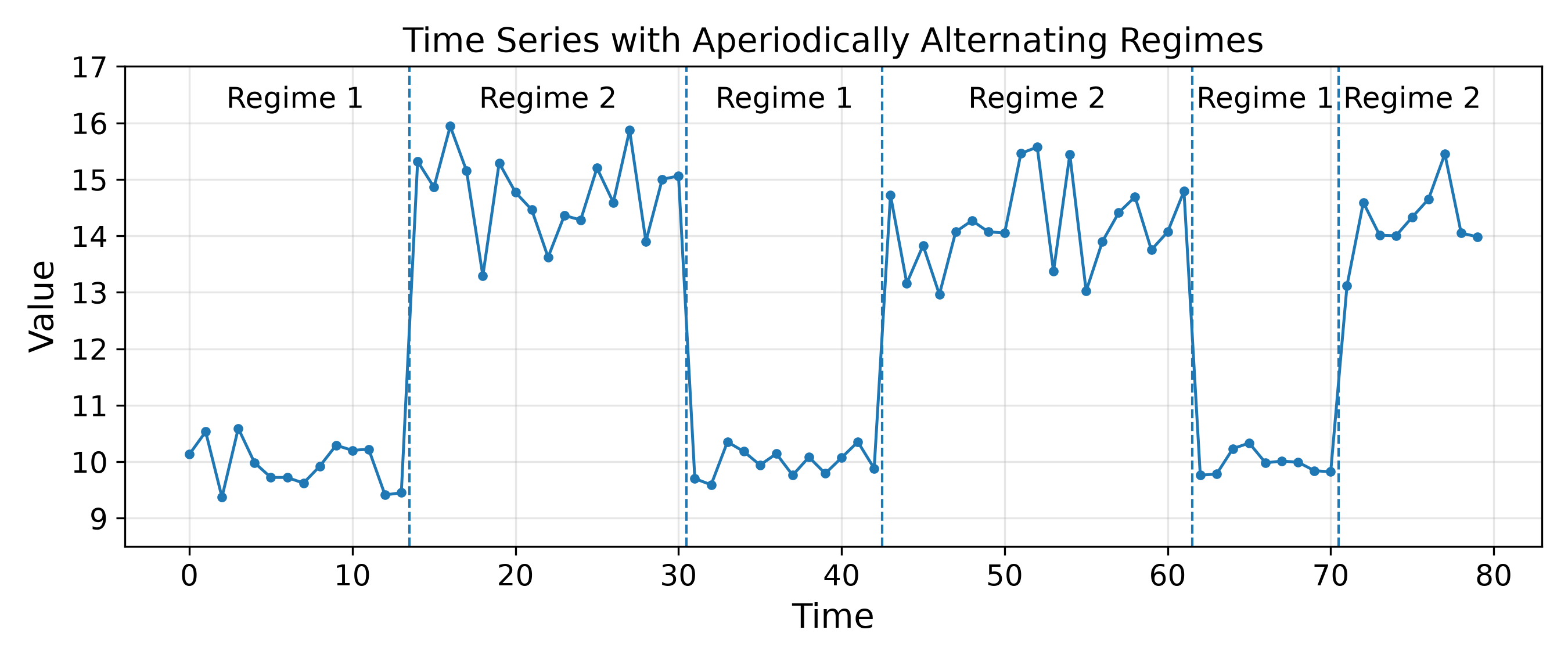
Regime changes may be caused by external events, operational modes, or recurring environmental conditions, and recognizing them is important because models that assume a single stationary process often perform poorly when multiple regimes are present. One approach is to detect regime changes (or change points) and split the time series into segments that are analyzed or modeled separately. The other approach is to use regime-switching models which explicitly model transitions between multiple regimes within a single framework. More generally, machine learning and neural network models may also learn different operating regimes implicitly when sufficient training data are available, although they do not explicitly represent regime changes unless specifically designed to do so.

Data Quality & Complexity

The data quality and complexity of a time series describe characteristics that affect the reliability, interpretability, and difficulty of analyzing the data. These include issues such as outliers, intermittent observations, high dimensionality, and scale or variables with different scales. Note that characteristics such as missing values or noise also refer to quality, but they are typically considered part of observation structure (i.e., how the data was observed and recorded); data quality & complexity describes how reliable or challenging the observed data are to analyze.

Outliers

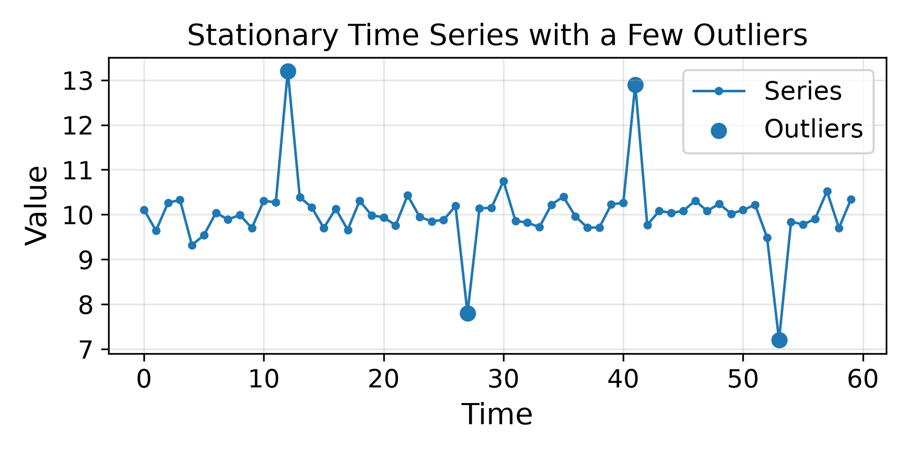
Outliers are observations that differ substantially from the typical behavior of a time series. They may arise from measurement or recording errors (cf. observation structure), but they can also represent genuine but rare events, such as equipment failures, extreme weather, or sudden market shocks.

Cause	Description	Example
Measurement error	Incorrect observations caused by faulty sensors or recording devices.	A temperature sensor briefly reports 200 °C instead of 20 °C.
Data entry or processing error	Mistakes during data recording, transmission, or preprocessing.	An extra zero is added to a manually entered sales value.
Equipment malfunction	Temporary failure of a monitored system produces abnormal values.	A machine vibration sensor spikes during a mechanical fault.
Extreme natural events	Rare but genuine events outside the normal operating range.	Exceptionally high river levels during a major flood.
Human or operational events	One-time events lead to unusually large or small observations.	Retail sales surge during a promotional campaign.
External shocks	Unexpected external events abruptly affect the observed process.	Stock prices drop sharply following unexpected economic news.

Outliers require careful interpretation because they are not always undesirable. If they result from measurement errors or data corruption, they can distort statistical analyses, bias model estimates, and reduce forecasting accuracy, making preprocessing necessary. However, outliers may also correspond to rare but meaningful events, such as equipment failures, fraudulent transactions, disease outbreaks, or extreme weather. In these applications, identifying such unusual observations is often the primary objective of the analysis, making outlier detection an important task in time series analysis.

To give an example, the plot below shows a basic stationary time series but which contains several outliers. Let's assume the observation a the readings of an environmental sensor (e.g., temperature, humidity, air quality). Again, depending on the application, outliers may be noise due to faulty hardware or genuine readings that should trigger an alert.

Intermittency

Intermittency refers to a time series in which observations are frequently zero or absent for extended periods, with non-zero values occurring only occasionally and often irregularly. Such series arise when the underlying events themselves occur infrequently rather than because observations are missing. Intermittent time series are common in inventory management, maintenance, healthcare, and logistics; for example:

Cause	Description	Example
Low demand frequency	Events occur only occasionally.	Demand for rarely used aircraft spare parts.
Rare failures	Equipment operates normally most of the time, with infrequent failures.	Replacement of industrial machine components.
Emergency events	Incidents occur sporadically and unpredictably.	Daily ambulance dispatches to a rural area.
Seasonal or event-driven demand	Activity is concentrated around specific events or seasons.	Sales of fireworks outside New Year's celebrations.
Rare natural phenomena	Observations correspond to infrequent environmental events.	Daily occurrences of earthquakes above a certain magnitude.
Infrequent transactions	Events are generated only when transactions occur.	High-value property sales in a small town.

Such time series are challenging to forecast because conventional methods often assume more continuous patterns of activity. As a result, specialized forecasting methods are frequently required to model both the timing and magnitude of intermittent events.

High Dimensionality

High dimensionality refers to time series datasets that contain a large number of variables, entities, or both, resulting in many simultaneous time-dependent observations (cf. dimensionality section above). Common practical examples include:

Cause	Description	Example
Many measured variables	A single system is monitored using numerous sensors or features.	Hundreds of sensors measuring temperature, pressure, vibration, and flow in a manufacturing plant.
Many entities	The same variable is recorded for a large number of similar entities.	Daily sales for thousands of products in a retail chain.
Large sensor networks	Data are collected simultaneously from many distributed devices.	Air quality measurements from hundreds of environmental monitoring stations.
Multimodal monitoring	Different types of measurements are collected for the same process.	Patient monitoring combining ECG, blood pressure, oxygen saturation, respiration, and temperature.
Large-scale financial markets	Many assets are observed over time.	Minute-by-minute prices for thousands of stocks in a stock exchange.
IoT and cyber-physical systems	Large numbers of connected devices continuously generate time series.	Smart city infrastructure monitoring traffic, energy consumption, parking occupancy, and weather sensors.

High-dimensional time series increase computational complexity and often exhibit redundant or correlated information, making tasks such as modeling, forecasting, and interpretation more challenging. As a result, dimensionality reduction, feature selection, or specialized high-dimensional models are often employed.

Scale

Scale refers to the size of a time series dataset in terms of the number of observations, the number of variables, or the number of individual time series it contains. Modern applications often generate massive amounts of temporal data from sensors, IoT devices, financial markets, or online services, resulting in datasets that require efficient storage, processing, and modeling techniques.

Application	Typical Scale	Example
Wearable sensor	Thousands of observations	Heart rate measured every second for one day.
Industrial monitoring	Millions of observations	Hundreds of sensors sampled every second over several months.
Retail analytics	Thousands of time series	Daily sales for thousands of products across many stores.
Financial markets	Millions to billions of observations	Tick-by-tick prices for thousands of financial instruments.
Smart city	Millions of time series	Continuous measurements from traffic, weather, energy, and environmental sensors.
Cloud services	Billions of observations	Server performance metrics collected from thousands of machines every few seconds.

Large-scale time series pose computational challenges for data preprocessing, visualization, model training, and forecasting, often motivating the use of distributed computing, online algorithms, or scalable machine learning methods. Note that this notion of scale is complementary to high dimensionality:

• High dimensionality concerns the number of variables (features) measured at each time step
• Scale concerns the overall size of the dataset, including the number of observations, the number of time series, or both

For example, a dataset with one billion hourly temperature measurements from a single sensor is large-scale but low-dimensional, whereas a dataset containing $10,000$ physiological variables measured for a single patient is high-dimensional but not necessarily large-scale. Many modern applications are both high-dimensional and large-scale.

---

Algorithms & Models

A wide variety of approaches have been developed for time series analysis, each based on different assumptions about the underlying temporal dynamics and designed to address different forecasting scenarios. Broadly, these approaches can be grouped into four major model families: classical statistical models, state space models, traditional machine learning models, and deep learning models. Each family differs in how it represents temporal dependencies, the type of input data it requires, its modeling assumptions, and its suitability for different types of time series.

Again, keep in mind that the goal is not to provide a comprehensive treatment of the numerous individual models within each family, but rather to introduce their fundamental concepts and underlying intuition. By discussing the basic principles, typical applications, and general advantages and disadvantages of each model family, this section establishes a high-level understanding of the available approaches and provides a conceptual basis for comparing them and selecting appropriate models for different time series analysis tasks.

Classical Statistical Models

Classical statistical models are among the earliest and most widely used approaches for time series analysis. Their basic assumption is that future values can be predicted from the historical behavior of the time series, often by modeling autocorrelation, trends, and seasonal patterns. The basic concept of classical statistical models is to describe the underlying temporal structure of the data using a predefined mathematical formulation with interpretable parameters. For example, autoregressive models predict future observations as a linear combination of previous values, while moving average models account for the influence of past forecast errors. More advanced models combine these concepts with differencing to model non-stationary series and incorporate seasonal patterns.

All classical statistical work directly on the original time series and assume regularly sampled data. For example, given our small univariate time series of a patient's hourly heart rate with $5$ observations (i.e., heart rate readings), a statistical model will receive as input:

$$\large \mathbf{x} = [72, 75, 74, 78, 76] $$

The different classical statistical models mainly differ in which temporal patterns they assume exist in the data and how they model them. While all of them operate directly on the time series, each model is designed to capture different aspects of temporal dependence. The table below provides a general overview of different models.

Model	Basic idea	Best suited for
Autoregressive (AR)	Predicts the current value as a linear combination of previous observations.	Stationary series with autocorrelation.
Moving Average (MA)	Models the current value as a function of previous random forecast errors (shocks).	Stationary series where short-term random disturbances influence future observations.
Autoregressive Moving Average (ARMA)	Combines AR and MA components to model both persistence and random shocks.	Stationary time series with both autocorrelation and noise effects.
Autoregressive Integrated Moving Average (ARIMA)	Extends ARMA by applying differencing to remove trends and achieve stationarity.	Non-stationary series with trends.
Seasonal ARIMA (SARIMA)	Extends ARIMA with additional seasonal autoregressive, differencing, and moving average components.	Time series with recurring seasonal patterns.
Exponential Smoothing (ETS)	Forecasts by exponentially weighting recent observations and explicitly modeling level, trend, and seasonality.	Time series with trend and/or seasonality, especially when recent observations should receive greater weight.

You can see from the table above, you can see that the progression of these models can be viewed as adding increasing levels of complexity. We can also illustrate this progression by given an intuition what the the different models are able to capture:

• AR: "Today's value depends on previous values."
• MA: "Today's value depends on previous prediction errors."
• ARMA: "Today's value depends on both previous values and previous errors."
• ARIMA: "If the series has a trend, first remove it by differencing, then apply ARMA."
• SARIMA: "Additionally account for recurring seasonal behavior."
• ETS: "Instead of modeling autocorrelation directly, decompose the series into level, trend, and seasonal components, while giving more weight to recent observations."

To give an example, let's consider Autoregressive Moving Average (ARMA). ARMA combines an autoregressive (AR) component, which models the dependence on previous observations, and a moving average (MA) component, which models the influence of previous random shocks (forecast errors). The mathematical formulation of an $\text{ARMA}(p,q)$ model is:

$$\large x_t = c + \sum_{i=1}^{p}\phi_i x_{t-i} + \varepsilon_t + \sum_{j=1}^{q}\theta_j \varepsilon_{t-j}, $$

where:

• $x_t$ = observation at time $t$,
• $c$ = constant (intercept),
• $\phi_i$ = autoregressive (AR) coefficients,
• $p$ = order of the AR component,
• $\theta_j$ = moving average (MA) coefficients,
• $q$ = order of the MA component,
• $\varepsilon_t$ = white noise (random error) at time $t$.

For example, $\text{ARMA}(1,1)$ is a so-called first-order ARMA model. With $p=q=1$, the general ARMA formula form above simplifies to:

$$\large x_t = c + \phi x_{t-1} + \varepsilon_t + \theta \varepsilon_{t-1} $$

Here:

• $x_{t-1}$ captures the persistence of the time series,
• $\varepsilon_{t-1}$ captures the effect of the previous forecast error,
• $\varepsilon_t$ represents the new random disturbance.

For instance, if yesterday's heart rate was unusually high and the previous forecast underestimated it, the AR term accounts for the persistence of the elevated heart rate, while the MA term adjusts the prediction based on the previous forecasting error.

Training an ARMA model consists of estimating the model parameters which are typically estimated using Maximum Likelihood Estimation (MLE) or nonlinear optimization techniques that iteratively search for the parameter values that maximize the likelihood of the observed time series. During this process, the model repeatedly computes one-step-ahead predictions and the corresponding forecast errors until the parameter estimates converge. Once trained, the estimated ARMA model can be used to recursively forecast future observations based on previous values and estimated prediction errors.

Given this mathematical formulation, an ARMA model predicts the current observation as a linear combination of previous observations and previous forecast errors, making it suitable for modeling stationary time series that exhibit both temporal dependence and correlated random disturbances. In contrast, ARMA models generally fail to adequately represent non-stationary time series that exhibit trends, changing variances, or seasonal behavior, because these characteristics violate the stationarity assumption. For such series, extensions such as ARIMA, which incorporates differencing to remove trends, or SARIMA, which additionally models seasonal patterns, are typically more appropriate. Moreover, because ARMA models assume linear relationships between observations, they may also struggle to capture highly nonlinear temporal dynamics commonly encountered in complex real-world time series.

Despite recent advances in machine learning and deep learning models, classical statistical models are still very popular for time analyzing time series for wide range of important reasons, particularly:

• Specifically designed for time series, directly modeling temporal dependencies such as autocorrelation, trends, and seasonality (depending on the exact model)
• Require no feature engineering, as they operate directly on the original sequential data
• Highly interpretable, with model parameters having clear statistical meanings (e.g., autoregressive and moving average coefficients)
• Perform well on small to moderate-sized datasets, often outperforming more complex machine learning models when data are limited
• Computationally efficient, making model fitting and forecasting relatively fast
• Well-established theoretical foundation, providing statistical inference, confidence intervals, and well-understood model diagnostic

However, the assumption and restrictions come with downsides, depending on the type of time series to be analyzed. The list below outlines the main disadvantages that need to be considered for practical application of these models:

• Often assume stationarity, requiring preprocessing steps such as differencing or detrending for non-stationary series.
• Assume linear relationships, limiting their ability to model complex nonlinear temporal dynamics
• Typically require regularly sampled data, making them less suitable for irregularly spaced observations without preprocessing
• Have limited ability to incorporate many external predictors, particularly compared with modern machine learning methods
• Require manual model selection, including choosing appropriate model orders and validating underlying assumptions
• May perform poorly on highly complex or high-dimensional forecasting tasks, where deep learning or advanced machine learning models can better capture intricate temporal patterns

State Space Models

The intuition behind state space models is that the observed time series is often only an indirect and noisy measurement of an underlying system whose true state cannot be observed directly. Instead of modeling the observations themselves, state space models assume that a set of hidden (latent) variables, called the state, summarizes all relevant information about the system at a given point in time. This hidden state evolves over time according to the system's dynamics, while the observations are generated from the current state and are subject to measurement noise.

A simple analogy is tracking the position of a moving car using GPS. The GPS measurements are noisy and may fluctuate even if the car moves smoothly. Rather than assuming that the noisy measurements represent the true position, a state space model estimates the car's hidden true position and velocity. As new observations become available, the model continuously updates its estimate of the hidden state (that car's true position and velocity), balancing the prediction from the system dynamics with the information contained in the new measurements.

For time series forecasting, the hidden state may represent quantities such as the underlying level, trend, seasonal effects, or other latent processes driving the observations. By estimating these components separately from measurement noise, state space models can produce more accurate forecasts and provide a structured interpretation of the temporal dynamics. This ability to infer an evolving hidden state distinguishes state space models from classical approaches, which model the observed time series directly rather than an underlying latent process.

The table below lists commonly used state space models for time series analysis:

Model	Description	Typical Applications
Local Level Model	Models a time-varying level (random walk).	Slowly changing signals, sensor measurements.
Local Linear Trend Model	Extends the local level model with a changing trend.	Economic indicators, demand forecasting.
Structural Time Series (STS) Models	Represent the series as latent components such as level, trend, seasonality, and cycles.	General forecasting, decomposition, economics.
Dynamic Linear Models (DLMs)	General linear state space models that can include regression effects and time-varying parameters.	Forecasting with external variables.
Kalman Filter Models	Linear Gaussian state space models estimated recursively using the Kalman filter.	Tracking, navigation, finance, forecasting.
Hidden Markov Models (HMMs)	Assume the hidden state is discrete rather than continuous.	Regime switching, speech recognition, activity recognition.
Switching State Space Models	Combine continuous state space models with discrete regime changes.	Financial markets, fault detection.
Bayesian State Space Models	Estimate latent states and parameters within a Bayesian framework.	Uncertainty quantification, probabilistic forecasting.

For the most part, state space models generally operate directly on the original time series just like classical statistical approaches. For example, when using our small example time series of a patient's hourly heart rate,

Timestamp	Heart Rate (bpm)
2025-01-01 08:00	72
2025-01-01 09:00	75
2025-01-01 10:00	74
2025-01-01 11:00	78
2025-01-01 12:00	76

a state space model, like any classical statistical model, simply receives:

$$\large \mathbf{x} = [72, 75, 74, 78, 76] $$

together with the observation times (if required). It internally estimates the latent state at each time step:

$$\large \begin{align} \text{Observed series:}\quad & 72 \rightarrow 75 \rightarrow 74 \rightarrow 78 \rightarrow 76\\[1em] \text{Hidden state:}\quad & x_1 \rightarrow x_2 \rightarrow x_3 \rightarrow x_4 \rightarrow x_5 \end{align} $$

The state equation propagates the hidden state over time, while the observation equation links each hidden state to the observed value. The important point is that the hidden states are not observed and are therefore not uniquely determined. Their values depend on the specific state space model (e.g., local level, local linear trend, structural model) and the estimated model parameters. The hidden states represent the model's best estimate of the underlying process, not the observations themselves.

For example, consider a Local Level Model, where the hidden state represents the patient's true heart rate and the observations contain measurement noise (see the example above):

$$\large \begin{aligned} z_t &= z_{t-1} + w_t \\ x_t &= z_t + v_t \end{aligned} $$

where $w_t \sim \mathcal{N}(0,Q),$ is the process noise and $v_t \sim \mathcal{N}(0,R)$ is the measurement noise. Omitting all the mathematical details here, let's assume we use a Kalman filter, the standard estimation algorithm for a local level model, yielding the following hidden states $x_t$ given the observation $x_t$ (i.e., the measured heart rate of the patient):

Timestamp	Observation $x_t$	Estimated State $z_t$
2025-01-01 08:00	72	72.0
2025-01-01 09:00	75	73.4
2025-01-01 10:00	74	73.7
2025-01-01 11:00	78	75.6
2025-01-01 12:00	76	75.8

Notice that the estimated states are smoother than the observations. Rather than jumping directly from 74 to 78 and back to 76, the hidden state evolves more gradually because the model assumes the underlying heart rate changes smoothly while the measurements are noisy.

The intuition is that the hidden state asks:

"What is the patient's true* physiological heart rate right now?"*

whereas the observation is:

"What did the sensor measure?"

If the sensor is noisy, the hidden state filters out these fluctuations.

This illustrates an important aspect of state space models: the hidden state does not have to resemble the observations directly. It can consist of multiple latent variables (e.g., level, trend, seasonal effects, cycle, or other unobserved quantities) that together describe the system's dynamics. The observed time series is then viewed as a noisy manifestation of these underlying latent states.

State space models are a popular approach for time series solutions as they offer several core benefits, including:

• Model latent states explicitly, providing estimates of unobserved components such as level, trend, seasonality, or system dynamics
• Provide interpretable models, as the hidden states often correspond to meaningful physical or statistical quantities
• Effectively handle noisy and missing observations through recursive state estimation methods such as the Kalman filter
• Support online (recursive) estimation, making them suitable for real-time monitoring and forecasting as new observations become available
• Offer a flexible modeling framework, accommodating time-varying parameters, external covariates, and probabilistic forecasting with uncertainty estimates

On the hand, various disadvantages of state space models also need to be considered when using them for time series analysis in practice:

• Require explicit model specification, including assumptions about the latent state dynamics and observation process
• Depend on distributional assumptions, with many classical approaches assuming linear Gaussian systems (although extensions exist for nonlinear and non-Gaussian settings)
• Can be mathematically and computationally complex, particularly for nonlinear, high-dimensional, or Bayesian state space models
• Require parameter estimation, including process and observation noise variances, which can be challenging for complex models or limited data
• May struggle to capture highly nonlinear relationships compared with modern deep learning approaches unless more sophisticated nonlinear state space models are used
• Model performance depends strongly on the appropriateness of the chosen state space formulation, making model selection and validation an important part of the analysis

Machine Learning Models

Although traditional machine learning models such as linear regression, random forests, support vector machines, and gradient boosting algorithms are not inherently designed to process sequential data, they can still be effectively applied to time series forecasting. Unlike specialized time series models, these algorithms treat observations as independent and therefore cannot directly capture temporal dependencies. To overcome this limitation, the time series must first be transformed into a cross-sectional dataset through a feature engineering process. In this transformed dataset, each observation is represented by a set of explanatory variables that encode information about the historical behavior of the series.

Feature engineering enables traditional machine learning models to exploit temporal patterns by creating informative predictors from the original time series. Commonly used features include lag variables, which represent previous observations, rolling statistics such as moving averages or rolling standard deviations to capture local trends and volatility, and calendar-based variables such as day of the week, month, season, or holiday indicators to account for recurring seasonal effects. Additional features, such as differences, growth rates, or external explanatory variables, can further enhance predictive performance. By converting the sequential data into a structured tabular format, traditional machine learning models can leverage their strong predictive capabilities while effectively incorporating the temporal information contained in the original time series.

To give a simple example, consider again the small univariate time series for a patients hourly heart rate we have seen before:

Timestamp	Heart Rate (bpm)
2025-01-01 08:00	72
2025-01-01 09:00	75
2025-01-01 10:00	74
2025-01-01 11:00	78
2025-01-01 12:00	76

Using $3$ lag features and a rolling mean with a window size of 3, the time series can be transformed into the following cross-sectional dataset. Here, the target variable is the current heart rate, while the features are derived from previous observations.

Timestamp	Target (Heart Rate)	Lag 1	Lag 2	Lag 3	Rolling Mean (3)
2025-01-01 08:00	72	–	–	–	–
2025-01-01 09:00	75	72	–	–	–
2025-01-01 10:00	74	75	72	–	73.67
2025-01-01 11:00	78	74	75	72	75.67
2025-01-01 12:00	76	78	74	75	76.00

The rolling mean is computed over the current observation and the two preceding observations. For example, at 11:00, the rolling mean is:

$$\large \frac{75 + 74 + 78}{3} = 75.67 $$

Side note: In practice, to avoid data leakage when forecasting, the rolling mean should be computed only from past observations. The feature table would therefore typically use a lagged rolling mean, i.e., the mean of the previous three heart rate measurements (excluding the current target value).

Several traditional machine learning models have been successfully applied to time series forecasting after appropriate feature engineering. Linear regression is commonly used as a simple and interpretable baseline, while decision trees and ensemble methods such as Random Forests, Gradient Boosting Machines (GBM), XGBoost, LightGBM, and CatBoost are widely adopted because they can capture complex, nonlinear relationships and interactions among engineered features. Support Vector Regression (SVR) is effective for modeling nonlinear patterns, particularly in smaller datasets, whereas k-Nearest Neighbors (k-NN) can exploit similarities between historical observations. These models are popular because they are flexible, computationally efficient, and capable of incorporating a wide range of engineered features, including lag variables, rolling statistics, calendar effects, and external covariates. Consequently, they often achieve high forecasting accuracy while providing greater flexibility than traditional statistical time series models in handling nonlinearities and multiple explanatory variables.

Using traditional machine learning models has several practical advantages, mainly:

• Can model complex nonlinear relationships that are difficult for many classical statistical models to capture (assuming nonlinear models)
• Easily incorporate multiple predictor variables, including lag features, rolling statistics, calendar variables, and external covariates
• Often achieve high predictive accuracy when sufficient historical data and well-engineered features are available
• Are flexible and scalable, making them suitable for a wide range of forecasting problems and large datasets
• Ensemble methods are generally robust to noise and outliers

On the other hand, traditional machine learning models come with some intrinsic challenges and disadvantages as well:

• Require extensive feature engineering to transform the time series into a tabular dataset
• Do not explicitly model temporal dependencies, such as autocorrelation, trend, or seasonality
• Are often less interpretable than classical statistical models, making it more difficult to understand the forecasting process
• Typically require larger training datasets to achieve good predictive performance
• May be prone to overfitting without appropriate feature selection, regularization, and time-aware validation.
• Usually involve a more complex modeling workflow beyond feature engineering, including hyperparameter tuning, and careful cross-validation

Deep Learning Models

Unlike traditional machine learning models, various deep learning models are inherently designed to process sequential data and can therefore be applied directly to time series analysis without extensive manual feature engineering. These mainly include architectures such as

• Recurrent Neural Networks (RNNs) and its variants Long Short-Term Memory (LSTM) networks and Gated Recurrent Units (GRUs)
• Temporal Convolutional Networks (TCNs)
• Transformers

These models are capable of learning temporal dependencies, trends, and seasonal patterns directly from raw sequential data. By automatically extracting relevant representations and capturing both short- and long-term dependencies, deep learning models can effectively model complex nonlinear dynamics in time series, making them particularly well suited for forecasting tasks involving large datasets and intricate temporal relationships.

Let's again use the small time series of a patient's heart rate and convert it into a datasata for training an LSTM for forecasting. Using a window size of $3$, each training example contains three consecutive heart-rate observations as the input sequence, and the following observation as the prediction target — since our example time series has only $5$ observation, this gives us only $2$ training sampels of size $3$.

Training Sample	Input Sequence (X)	Target (y)
1	[72, 75, 74]	78
2	[75, 74, 78]	76

For an LSTM, the batched input is typically arranged in the shape $(\text{num\_samples, time\_steps, num\_features})$. Since there are two samples, three time steps, and one feature, the input shape is $(2, 3, 1)$:

$$\large X = \begin{bmatrix} [72], [75], [74] \\ [75], [74], [78] \end{bmatrix}, \qquad y = \begin{bmatrix} 78 \ 76 \end{bmatrix}. $$

Each sequence therefore uses the previous three hourly heart-rate measurements to forecast the heart rate in the next hour. For a GRU or a (Vanilla) RNN, the format of the dataset would be exactly the same — after all, they are all "only" variants of Recurrent Neural Networks.

In fact, we can also use this format to train a Temporal Convolutional Network (TCN) as well as a Transformer model (more specifically, a encoder-only Transformer model). All models learns from fixed-length input sequences of historical observations, so the sliding window approach is the same. The main difference lies in how the models processes the sequence internally:

• LSTM: Sequential processing with recurrent memory cells
• TCN: Parallel processing using causal 1D convolutions
• Transformer: Parallel processing using self-attention with positional encodings to preserve temporal order

Note that deep learning models such as Multilayer Perceptrons (MLPs) that are not inherently designed to process sequential data can also be used for time series analysis. Of course, such models then again require a feature engineering step in which the time series is transformed into a tabular dataset using features such as lag variables, rolling statistics, calendar variables, and other engineered predictors. Once the sequential data have been converted into this cross-sectional representation, MLPs can be trained to learn complex nonlinear relationships between the engineered features and the target variable, making them a viable approach for time series forecasting.

The capacity and flexibility of deep learning models offer several advantages for time series analysis; most importantly:

• Designed for sequential data, enabling them to model temporal dependencies directly without extensive manual feature engineering
• Automatically learn feature representations from raw time series, reducing the need for handcrafted features such as lag variables and rolling statistics
• Capture complex nonlinear relationships and intricate temporal patterns that may be difficult for statistical or traditional machine learning models to represent
• Can learn both short-term and long-term dependencies, particularly with architectures such as LSTMs, TCNs, and Transformers
• Scale well to large datasets and high-dimensional multivariate time series.
• Can be adapted to a wide range of forecasting tasks, including multistep, multivariate, and probabilistic forecasting

In contrast, their capacity and complexity also introduce various practical challenges, which make deep learning models often the best or preferred choice for many uses cases:

• Typically require large amounts of training data to achieve good generalization and outperform simpler models
• Are computationally expensive, requiring greater training time, memory, and often specialized hardware such as GPUs
• Involve complex model architectures and numerous hyperparameters, making model selection and tuning more challenging
• Are generally less interpretable than statistical and many traditional machine learning models
• May be prone to overfitting, particularly when training data are limited or model complexity is high
• Often provide limited performance gains on small or simple datasets, where classical statistical or traditional machine learning models may perform equally well or better.

Summary & Comparison

Classical statistical models, state space models, machine learning models, and deep learning models make different assumptions, and have many different capacities but also limitations. The table below therefore provides a general comparison of those $$ 4 approaches. This comparison emphasizes that the four model families differ not only in predictive capability but also in how they represent temporal information, how they expect the input data to be formatted, their interpretability, and their computational complexity. These criteria provide a natural basis for comparing forecasting approaches in a thesis.

Criterion	Classical Statistical Models	State Space Models	Traditional Machine Learning	Deep Learning
Primary examples	AR, MA, ARIMA, SARIMA, ETS	Local Level, DLM, STS, Kalman Filter	Linear Regression, Random Forest, XGBoost, SVR	MLP, LSTM, GRU, TCN, Transformer
Designed for sequential data	Yes	Yes	No	Mostly (except MLP)
Input data	Original time series	Original time series	Feature-engineered tabular data	Sequential windows (LSTM, TCN, Transformer) or engineered features (MLP)
Feature engineering required	No	No	Yes	Usually no (except MLP)
Models temporal dependencies	Directly through autoregressive and seasonal components	Through latent state evolution	Indirectly via engineered features	Directly through recurrent, convolutional, or attention mechanisms
Handles nonlinear relationships	Limited	Limited (linear models) to moderate (nonlinear extensions)	Yes	Yes
Interpretability	High	High	Moderate	Low
Data requirements	Small to moderate datasets	Small to moderate datasets	Moderate to large datasets	Large datasets
Computational complexity	Low	Low to moderate	Moderate	High
Handles missing/noisy observations	Limited	Excellent	Limited	Limited
Supports online/recursive updating	Limited	Excellent	Generally no	Possible but uncommon
Typical application	Forecasting stationary or seasonal series	Dynamic systems, filtering, forecasting	Tabular forecasting problems with engineered features	Complex, nonlinear, high-dimensional forecasting

Given the different assumptions and requirements, selecting an appropriate forecasting model requires first understanding the characteristics of the underlying time series, as different modeling approaches are suited to different temporal patterns and data properties. Important characteristics include the presence of trends, seasonality, autocorrelation, non-stationarity, missing values, noise, nonlinear relationships, structural changes, and the availability of external explanatory variables. For example, classical statistical models are well suited to stationary or seasonal series with linear dependencies, whereas machine learning and deep learning models are often preferred for complex nonlinear patterns or high-dimensional data.

In practice, the characteristics of a time series are typically identified through a combination of exploratory data analysis (EDA) and statistical diagnostics. This process commonly begins with visual inspection of the time series to identify trends, seasonal patterns, outliers, and structural breaks. Statistical techniques such as autocorrelation (ACF) and partial autocorrelation (PACF) plots are then used to assess temporal dependencies, while stationarity tests, such as the Augmented Dickey-Fuller (ADF) or KPSS test, help determine whether preprocessing steps such as differencing are required. Additional analyses may include decomposition into trend and seasonal components, distributional analysis, and the assessment of missing values or irregular sampling. Together, these exploratory and statistical analyses provide valuable insights into the data and guide the selection of an appropriate forecasting model and preprocessing strategy.

---

Summary

In this notebook, we introduced the fundamental concepts of time series analysis and highlighted why temporal data play a central role in many scientific and industrial applications. We discussed how time series differ from conventional data by exhibiting temporal dependencies and explored the broad range of tasks they support, including understanding historical behavior, monitoring evolving systems, and predicting future outcomes.

We also examined the diverse characteristics of time series, including regular and irregular sampling, trends, seasonality, cycles, structural changes, regimes, additive and multiplicative behavior, and anomalies. Recognizing these properties is an important first step toward selecting appropriate analytical techniques and interpreting temporal data correctly. In addition, we provided an overview of commonly used methods and models for time series analysis, illustrating the variety of approaches available for different data characteristics and analytical objectives.

The purpose of this notebook was not to provide an exhaustive treatment of these topics, but rather to establish a conceptual foundation and common terminology. Many of the methods introduced here involve rich theoretical foundations, practical considerations, and specialized algorithms that extend well beyond the scope of an introductory overview.

This notebook should therefore be viewed as a starting point for further exploration of time series analysis. A solid understanding of the concepts and terminology presented here provides the basis for studying more advanced topics, including statistical time series models, state-space models, probabilistic forecasting, deep learning approaches, and domain-specific applications involving complex temporal data.