Disclaimer: This Jupyter Notebook contains content generated with the assistance of AI. While every effort has been made to review and validate the outputs, users should independently verify critical information before relying on it. The SELENE notebook repository is constantly evolving. We recommend downloading or pulling the latest version of this notebook from Github.
Transformers — Basic Architecture
The Transformer architecture, introduced in the groundbreaking paper "Attention is all you Need" in 2017, marked a fundamental shift in the design of deep learning models for sequence data. Unlike traditional Recurrent Neural Networks (RNNs) that process input sequentially, Transformers use a fully attention-based mechanism that enables parallel processing of entire sequences. This architectural innovation eliminated the inherent limitations of RNNs, such as difficulty handling long-range dependencies and slower training times due to their sequential nature.
One of the key characteristics that sets Transformers apart is the attention mechanism, which allows the model to dynamically weigh the relevance of different words in a sequence when generating representations. This enables the Transformer to capture global context effectively, regardless of the position of words in a sentence. In contrast, RNNs often struggle with maintaining context over long sequences due to vanishing gradients, and they typically require mechanisms like LSTM or GRU units to cope. Moreover, because Transformers do not rely on recurrence, they benefit greatly from GPU acceleration through parallelism, leading to more efficient training on large datasets.
Transformers have quickly become the foundation for many state-of-the-art models in natural language processing (NLP), computer vision, and even protein structure prediction. Models like BERT, GPT, T5, and Vision Transformers (ViTs) are all built on the Transformer architecture. Their success has revolutionized applications such as machine translation, text summarization, image classification, and code generation. The flexibility, scalability, and performance of Transformers have made them the go-to model for a wide range of tasks across AI and ML.
Given their dominance and versatility, understanding Transformers is essential for anyone looking to work in modern AI and ML. As the field continues to evolve, more applications are adapting the Transformer framework, not only because of its superior accuracy but also due to its adaptability across different data modalities. Whether you are interested in building chatbots, recommendation systems, or autonomous agents, a solid grasp of Transformer principles will provide a crucial foundation.
Setting up the Notebook
Make Required Imports
This notebook requires the import of different Python packages but also additional Python modules that are part of the repository. If a package is missing, use your preferred package manager (e.g., conda or pip) to install it. If the code cell below runs with any errors, all required packages and modules have successfully been imported.
import torch
import torch.nn as nn
from src.models.neural.transformer import MultiHeadAttention
Preliminaries
Before introducing you to the Transformer architecture, there are a few preliminary comments to outline the scope of this notebook:
Transformer rely on important concepts such as attention, masking, and positional encodings. While these topics will be briefly covered in this notebook, we recommend to check out the separate notebooks providing a deep dive into each of this topics
To make all visualizations, examples, and descriptions easier to understand, we assume that any input text is tokenized into proper words. Note that practical Transformer-based models typically rely on subword-based tokenizers (e.g., Byte-Pair Encoding, WordPiece).
With these clarifications out of the way, let's get started...
Generate Example Data
Throughout this notebook, we will actually implement a basic Transformer architecture step-by-step from scratch to better understand the individual components and how they work together. To this end, the code cell below creates two random tensors to mimic a machine translation task: SOURCE is the batch of sequences with the embedding vectors for all words in the source language; similarly, TARGET is the batch of sequences with the embedding vectors for all words in the target language. The size of both batches is $32$ and the length of each embedding vector is $d_{model} = 512$. In the Transformer architecture, $d_{model}$ refers to the dimensionality of the input and output embeddings as well as the hidden representations throughout the model. It defines the size of the vectors used to represent each word (more precisely: each token) in the sequence, and it remains constant across all layers of the encoder and decoder. The relevance of $d_{model}$ will be properly explained when explaining the overall architecture.
batch_size, d_model = 32, 512
seq_len_en, seq_len_de = 50, 60

torch.manual_seed(0)
SOURCE = torch.rand((batch_size, seq_len_en, d_model))
TARGET = torch.rand((batch_size, seq_len_de, d_model))

print(f"Shape of SOURCE tensor: {SOURCE.shape}")
print(f"Shape of TARGET tensor: {TARGET.shape}")
Shape of SOURCE tensor: torch.Size([32, 50, 512])
Shape of TARGET tensor: torch.Size([32, 60, 512])
Notice that both tensors differ with respect to the length of their sequences. This is realistic as there is no reason to assume that the same sentences but in different languages will contain the same number of words or tokens.
The Transformer Architecture
The figure below is taken from original Transformer paper "Attention is all you Need" and shows the overall Transformer architecture. The (full) Transformer is an encoder-decoder architecture — although different models may use only the encoder or only the decoder, as we will discuss at the end. If we assume an English-to-German machine translation task, the encoder and decoder served the following main purpose:
Encoder: The encoder's purpose is to read and understand the input sentence in the source language and convert it into a rich, contextualized representation. It does this by processing the input tokens through multiple layers of self-attention and feedforward networks, allowing the model to capture relationships between words regardless of their positions in the sentence. This means each word's representation is informed not just by its local context but by the entire sentence, enabling the model to grasp the nuances of meaning and grammar. By the end of the encoder, the input sentence is transformed into a sequence of embeddings that encapsulate both the individual word meanings and their contextual relationships. These embeddings are then passed to the decoder.
Decoder: The transformer decoder generates the output — here: the translated sentence in the target language — one word at a time, using the contextual information encoded by the encoder. The decoder takes the encoder's output and combines it with the previously generated target word to predict the next word in the translation. Each decoder layer first uses self-attention to consider the previously generated words, then cross-attention to incorporate relevant information from the encoder's output, followed again by a feedforward network. This process enables the decoder to build a grammatically correct and semantically accurate translation, ensuring that the generated sentence not only reflects the original meaning but also conforms to the structure and vocabulary of the target language.
This encoder-decoder architecture makes the Transformer a powerful and versatile model. Although Transformers were originally designed for sequential data such as language, their core mechanism — attention — is not limited to text and can model relationships between any set of elements, regardless of modality. In the case of images, an image can be divided into smaller, fixed-size patches (e.g., 16x16 pixels), and each patch is flattened and treated like a "word" in a sequence.
Both the encoder and decoder are composed of the same core building blocks which we will cover throughout this notebook.
Multi-Head Attention
Attention is at the heart of the Transformer architecture because it enables models to dynamically focus on the most relevant parts of the input data when making predictions. Unlike traditional sequence models that process data step by step, the attention mechanism allows Transformers to weigh the importance of all input tokens simultaneously, regardless of their position. This ability to capture long-range dependencies and contextual relationships between tokens is crucial for understanding complex structures in language and other data types.
The core idea behind attention is that not all parts of an input are equally important for a given task. By computing attention scores, the Transformer determines which tokens contribute most to a given output, enabling more flexible and efficient learning. This mechanism not only boosts performance in tasks like machine translation and text summarization but also allows for massive parallelization, making training faster and more scalable compared to recurrent architectures.
In the following, we motivate and introduce the concept of attention on a fairly high level, focusing on its intended purpose and output. To fully understand the inner workings of the attention algorithm, we recommend going through the notebook dedicated to attention in Transformers. This notebook covers all involved computations in great detail using illustrative examples.
Motivation & Basic Idea
Neural networks can't work directly with nominal or symbolic data like raw text because they are designed to perform mathematical operations on numerical data. Textual data — such as words or tokens — are inherently symbolic and have no inherent numerical meaning or structure that a neural network can interpret or compute on. For example, the words "cat" and "dog" are just labels; without numerical encoding, a neural network has no way to compare them or recognize patterns.
Furthermore, symbolic data lacks the continuous, differentiable structure that neural networks require for training. Neural networks learn by adjusting weights through gradient descent, which relies on calculating gradients — a process that only makes sense for numerical inputs. By converting text into numerical vectors (like embeddings), we give the model inputs it can compute with, while also preserving useful information about word meaning and relationships. This transformation is essential for enabling learning and generalization from textual data.
As a consequence, basically neural network architectures that work with nominal or symbolic data have an embedding layer as their first layer. An embedding layer is a type of neural network layer that maps discrete input tokens, such as word indices, into continuous vectors of fixed size. It is essentially a learnable lookup table where each row corresponds to the embedding of a specific word or token in the vocabulary. When a token index is passed into the embedding layer, it returns the corresponding vector — a process similar to looking up a value in a dictionary based on a key.
An embedding layer associates the same word or token to the same (learnable) embedding vector. In other words, independent of the context — such as the surrounding words or sentence(s) — the same words always map to the same vector. To see why this may cause problem when it comes to understanding natural language, consider the following example sentence:
A light wind will make the traffic light collapse and light up in flames
Just by looking at the three occurrences of the word "light", we can see the issue that arises when encoding the same word using the same embedding vector. For one, all three occurrences of "light" serve a different syntactic function: first an adjective, then a noun, and lastly a verb. But even even with respect to the same syntactic function, the same word may have (very) different meanings. For example, a traffic light is arguably a very different thing compared to a torch light — or just the noun "light" in a sentence like "I saw the light at the end of the tunnel". In short, using the same embedding vector for "light" fails to capture the word's syntactic function and proper meaning. This is where attention comes in.
Attention Head
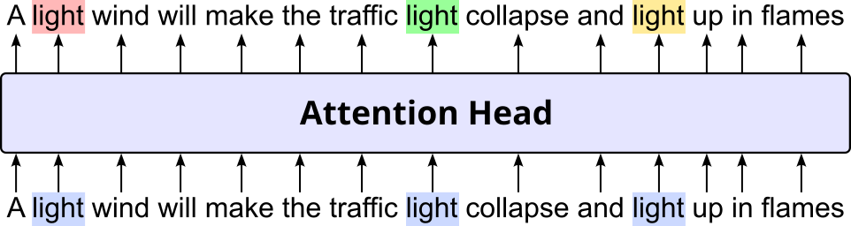
On an abstract level, an attention head in the Transformer architecture is a component that takes in a sequence of embedding vectors, "somehow" modifies them based on the context (i.e., all other words in the sequence), and returns the sequence of contextualized embedding vectors as output. The figure below illustrates this idea using the example sentence from above. The color-coding is supposed to convey that the input embedding vectors for the word "light" are the same, while its output embedding vectors will be different (i.e., contextualized).
The obvious question is of course now how exactly the attention head processes the input embedding vectors such that the output vectors are more likely to capture the syntax and semantics of a word. In very simple terms, the attention head computes the alignment between each word and all other words in the same or a different sequence (incl. the word itself). This alignment between embedding vectors is calculated based on the dot product. These alignments are then used to recompute the embedding vector of a word as the weighted sum of all other word embedding vectors — where the weights derive from the strength of the alignments. Regarding the context that is used to calculated the alignment between words, there are two main variants:
Self-attention: In self-attention, the alignment is calculated between words in the same sequence. For example, given our sentence "A light wind will make the traffic light collapse and light up in flames", self-attention computes the alignments between all pairs of embedding vectors. Both the encoder and decoder rely on self-attention to contextualize their input embedding vectors.
Cross-attention: In cross-attention, the input embedding vectors are align with words from a different sequence. Only the decoder has a cross-attention layer to align the decoder input (e.g., the sentence in the target language) with the encoder output (e.g., the sentence in the source language).
Multi-Head Attention
In practice, the Transformer architecture employs multiple attention heads — where $n_{heads}$ typically denotes the number of attention heads — instead of a single one to allow the model to capture diverse relationships and information from the input sequence simultaneously. By using multiple attention heads, the Transformer essentially gains multiple "perspectives" on the input. Each head operates independently, allowing different heads to focus on different aspects of the input. For example, one head might learn to identify syntactic dependencies (e.g., subject-verb relationships), another might focus on semantic relationships (e.g., recognizing synonyms or antonyms), and yet another might identify co-reference.
The outputs from these individual attention heads are then concatenated and linearly transformed, effectively combining these diverse perspectives into a single, more comprehensive representation. The figure below illustrates the combination of multiple attention heads (here: $n_{heads} = 3$) into a so-called multi-head attention (MHA) layer. Notice how the same input sequence is given to three independent attention heads and how their output is combined to the final sequence of contextualized embedding vectors.
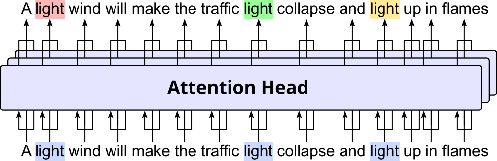
This ensemble-like approach not only allows the model to capture a wider range of linguistic phenomena but also makes the learning process more robust and efficient. It prevents any single attention pattern from dominating the learning, leading to a more nuanced and powerful understanding of the input sequence, which is critical for complex tasks like machine translation where intricate linguistic relationships need to be accurately captured.
We provide the class MultiHeadAttention that implements a multi-head attention layer for different values of $d_{model}$ and $n_{heads}$. In the code cell, we set $n_{heads} = 8$, and we already set the dimensionality of the input and output embeddings to $d_{model} = 512$.
n_heads = 8

mha = MultiHeadAttention(d_model, n_heads)
This layer accepts three tensors as input arguments. Without going into further detail here — again, you can check out the dedicated notebook about attention — the first tensor contains the input embeddings we want to contextualize; the other two tensors represent the context. This means that for self-attention, we pass the same tensor to all three arguments. The code cell below illustrates this for the self-attention layer in the encoder.
mha_out_self_attn = mha(SOURCE, SOURCE, SOURCE)

print(f"Shape of self-attention output: {mha_out_self_attn.shape}")
Shape of self-attention output: torch.Size([32, 50, 512])
Tensor mha_out_self_attn now contains the contextualized embedding vectors of SOURCE. Note that we do not care about the exact values but you should appreciate that the shape of the output tensor mha_out_self_attn is the same as for the input tensor SOURCE. We will see later why this is useful.
In contrast, the code cell below, shows an example for using the class to compute cross-attention between different sequences. Here, we mimic the cross-attention layer in the decoder, where we want to contextualize the embedding vectors of the sequence in the target language based on the embedding vectors of the sequence in the source language. Important: In the Transformer architecture, TARGET would be the output of the self-attention layer in the decoder, and SOURCE would be the output of the encoder. We only use our input tensor SOURCE and TARGET to illustrate the difference between self-attention and cross-attention.
mha_out_cross_attn = mha(TARGET, SOURCE, SOURCE)

print(f"Shape of cross-attention output: {mha_out_cross_attn.shape}")
Shape of cross-attention output: torch.Size([32, 60, 512])
Again, the shape of the output tensor is the same as the shape of the input tensor.
Take-away message: In a nutshell, multi-head attention aims to capture the relationship between words through calculating the pairwise alignment — typically using the dot product of embedding vectors — between all words in either the same sequence (self-attention) or different sequences (cross-attention). These alignment values are used to recalculate the input embedding vector of each word to better reflect its context (i.e., all other words this word was aligned with). The desired goal is that these contextualized embedding vectors better capture the semantic meaning of the words; for example:
"A light wind": here the embedding vector for "light" should be similar to the embeddings of other adjectives such as "soft", "mild", or "weak".
"the traffic light": ideally, the embedding for "light" should be similar to other objects (i.e., nouns) that give of light; this may include "lamp", "street light", "lamp pole", and similar concepts.
"light up in flames": in this context, the embedding for "light" should arguably similar to verbs such as "ignore", "burn", or "kindle".
Again, we provide a separate notebook that covers and goes through the attention mechanism in great detail, and we strongly recommend having a look at this notebook if you really want to understand how Transformers work.
Feed-Forward Network Layer
The feed-forward network (FFN) layer in the Transformer architecture serves the crucial role of transforming and enriching the representations produced by the attention mechanism. While attention allows the model to gather and integrate contextual information across a sequence, it operates primarily in the space of token interactions. The feed-forward layer, applied independently to each position in the sequence, acts as a position-wise fully connected neural network that further processes these contextualized representations. It introduces nonlinearity through activation functions like ReLU or GELU and enables the model to learn more complex transformations beyond what attention alone can achieve.
The FFN typically consists of two linear transformations with the nonlinear activation function in between. The input to the FFN is the output of the preceding multi-head attention layer (or the encoder's output in the decoder's second attention layer). The first linear layer expands the dimensionality of the token representation, effectively projecting it into a higher-dimensional space where more intricate features can be extracted. The activation function then introduces non-linearity, enabling the network to learn complex patterns that cannot be captured by linear transformations alone. Finally, the second linear layer projects the representation back to its original dimensionality. Mathematically, we can define the FFN therefore as:
where $\mathbf{x}$ is the input tensor, $\mathbf{W}_1$ and $\mathbf{W}_2$ are learnable weight matrices, $\mathbf{b}_1$ and $\mathbf{b}_2$ are learnable bias vectors. Here we assume ReLU as the applied nonlinear activation function as proposed in the original Transformer paper; although other activation functions are of course possible.
While the same FFN parameters (weights and biases) are applied to every token position, the transformation for each token is independent of the others. This "position-wise" nature allows for highly parallelizable computation, a key factor in the Transformer's efficiency. Essentially, the FFN acts as a local processing unit for each token, refining its representation based on the contextual information gathered by the self-attention mechanism. It adds depth and capacity to the model, allowing it to learn richer and more expressive representations of the input sequence.
This simple nature of the FFN layer makes it also very easy to implement. The code cell below implements the FNN layer as proposed in the original Transformer paper. This includes the use of the ReLU activation function between the two linear layers, as well as a default value of $d_{\mathit{ffn}} = 2,048$ for the output dimensionality of the first linear layer.
class FeedForwardNetwork(nn.Module):

    def __init__(self, d_model, d_ffn=2048):
        super().__init__()

        # Define basic Feed Forward Network as proposed in the original Transformer paper
        self.net = nn.Sequential(
            nn.Linear(d_model, d_ffn),
            nn.ReLU(),
            nn.Linear(d_ffn, d_model),
        )

    def forward(self, x):
        return self.net(x)
The choice of $d_{\mathit{ffn}}$ for the output dimension of the first linear transformation is related to the value of $d_{model}$ (here: $d_{model} = 512$). Typically, $d_{\mathit{ffn}} = 4\times d_{model}$ to allow the model to project input representations into a higher-dimensional space where more complex and expressive transformations can be learned. This design choice serves two main purposes:
Increased capacity and expressiveness: By expanding the input dimensionality (e.g., from $512$ to $2048$), the model creates a richer feature space that enables it to learn more nuanced patterns and interactions between elements of the representation. The subsequent non-linear activation function (like ReLU or GELU) operates more effectively in this expanded space, allowing the model to capture more abstract features.
Bottleneck structure for efficiency: After the non-linear transformation, the second linear layer projects the data back down to the original input size. This bottleneck structure is similar in spirit to architectures like autoencoders or residual networks, balancing model capacity with computational efficiency. Expanding and contracting the dimensionality allows the model to achieve high expressiveness without significantly increasing the overall size or runtime of the network.
In practice, this $4\times$ expansion has been found empirically to offer a good trade-off between performance and computational cost, and it has become a standard in many Transformer variants such as the original Vaswani et al. model and later versions like BERT and GPT.
Let's create an instance of the FeedForwardNetwork class to show its application; we go with the default argument d_ffn=2048:
d_ffn = 2048

ffn = FeedForwardNetwork(d_model, d_ffn=d_ffn)

print(ffn)
FeedForwardNetwork(
  (net): Sequential(
    (0): Linear(in_features=512, out_features=2048, bias=True)
    (1): ReLU()
    (2): Linear(in_features=2048, out_features=512, bias=True)
  )
)
As mentioned before — and as shown in the overall architecture (see above) — the FFN layer always receives as input the output of an multi-head attention layer; note that there are some additional steps involved, which we will cover later. Thus, as illustration, we give one of the example outputs from our multi-head attention implementation as input to the FFN; see the code cell below.
ffn_out = ffn(mha_out_self_attn)

print(ffn_out.shape)
torch.Size([32, 50, 512])
Unsurprisingly, since the FFN layer maps each embedding vector first from $d_{model}$ to $d_{\mathit{ffn}}$ and then back to $d_{model}$, the shapes of the input tensor and the output tensor are again the same. The values of the embedding vectors will naturally have changed, to hopefully represent richer and more nuanced word representations.
Encoder
With the multi-head attention layer and the feed-forward network layer, we now have the core components of both the Transformer encoder and decoder. In fact, the encoder and decoder are structurally quite similar, as we will see in the following. So let's start with the encoder.
Encoder Layer
A single encoder layer in the Transformer architecture is a fundamental building block that processes input sequences to capture contextual relationships between tokens. It primarily consists of two main sublayers: the multi-head self-attention mechanism and the feed-forward neural network. The figure below shows the part of the overall architecture that represents a single encoder layer.
Apart from the multi-head attention and feed-forward network layer, an encoder layer implements a series of additional concepts. We briefly outline these additional concepts below but omit a more detailed discussion here since they are not specific to the Transformer architecture; these concepts are common in many neural network architectures.
Layer normalization: Layer normalization is a technique used to stabilize and accelerate the training of neural networks by normalizing the inputs across the features of a single training example. It operates independently for each sample by computing the mean and variance of all features in a layer and using them to normalize the feature values. After normalization, the values are scaled and shifted using learned parameters, allowing the model to recover the original distribution if needed. The main purpose of layer normalization is to reduce internal covariate shift — the change in the distribution of inputs to a layer during training — which helps make the optimization process more stable and efficient. It is particularly useful in architectures like Transformers and recurrent neural networks, where batch sizes may vary or where dependencies exist within a single sequence rather than across batches. By ensuring consistent activation distributions, layer normalization improves convergence and performance in deep models.
Residual connections: Residual connections, also known as skip connections, are a fundamental architectural component in deep neural networks, notably popularized by Residual Networks (ResNets), and have since become a foundational component in models like Transformers. They work by creating a "shortcut" path that bypasses one or more layers, directly adding the input of a layer (or a block of layers) to its output. Notice in the figure above the two connections that bypass the multi-head attention layer and the feed-forward network layer. The main purpose of residual connections is to address the vanishing gradient problem and help train deep networks more effectively. By providing a shortcut for gradients to flow backward through the network, residual connections make it easier to optimize very deep architectures. They also allow layers to focus on learning small refinements (residuals) rather than complete transformations, which often leads to faster convergence and better performance.
Dropout: (not explicitly visualized in the figure above) Dropout is a regularization technique used in neural networks to prevent overfitting during training. It works by randomly "dropping out" (i.e., setting to zero) a fraction of the neurons in a layer during each forward pass. This means that during training, the network effectively samples from a larger ensemble of smaller networks, each with different architectures depending on which neurons are dropped at that moment. At test time, dropout is turned off, and all neurons are used, typically with their outputs scaled appropriately to maintain consistency. The main purpose of dropout is to improve the model’s generalization by reducing reliance on specific neurons or features. By forcing the network to learn redundant representations and preventing co-adaptation of neurons, dropout helps ensure that the model performs well not just on the training data, but also on unseen data. This makes it particularly effective in reducing overfitting, especially in deep or complex networks such as Transformers.
The class TransformerEncoderLayer in the code cell below implements a single encoder layer. Notice the multi-head attention block containing the multi-head attention layer itself, as well as the dropout and layer normalization, as well as the feed-forward network layer with its own dropout layer in layer normalization. The residual connections are represented by the addition of the output of a layer with its input (before applying layer normalization).
class TransformerEncoderLayer(nn.Module):

    def __init__(self, d_model, n_heads, d_ffn=2048, dropout=0.1):
        super().__init__()

        # MultiHeadAttention block
        self.mha1 = MultiHeadAttention(d_model, n_heads)
        self.dropout1 = nn.Dropout(dropout)
        self.norm1 = nn.LayerNorm(d_model)

        # FeedForwardNetwork block
        self.ffn = FeedForwardNetwork(d_model, d_ffn)
        self.dropout2 = nn.Dropout(dropout)
        self.norm2 = nn.LayerNorm(d_model)

    def forward(self, source):
        # MultiHeadAttentionBlock
        out1 = self.mha1(source, source, source) # self-attention
        out1 = self.dropout1(out1)               # dropout
        out1 = self.norm1(out1 + source)         # residual connection
        # FeedForward block
        out2 = self.ffn(out1)                    # feed-forward network (incl. nonlinearity)
        out2 = self.dropout2(out2)               # dropout
        out2 = self.norm2(out2 + out1)           # residual connection + layer normalization
        # Return final output
        return out2
We can now create a single transformer layer based on the values for $d_{model}$ and $n_{heads}$. We use the default values for $d_{\mathit{ffn}}$ and the dropout probability.
encoder_layer = TransformerEncoderLayer(d_model, n_heads)

#print(encoder_layer)  # quite verbose and not very important, but feel free to comment out to show network architecture
Assuming our machine translation task, the encoder layer will receive the batch containing all sequences representing the sentences in the source language as input. We can implement this, by simply passing tensor SOURCE to the encoder layer. Since we already know how the multi-head attention and the feed-forward network layer behaves, it is not surprising that the shape of the encoder output is the same as of the input.
encoder_layer_output = encoder_layer(SOURCE)

print(f"Shape of encoder layer output: {encoder_layer_output.shape}")
Shape of encoder layer output: torch.Size([32, 50, 512])
The fact that the tensor shapes remain the same has the obvious advantage that this makes it very easy to stack multiple encoder layers on top of each other.
Complete Encoder
The complete encoder is now simply a list of multiple encoder layers that are stacked upon each other, with $n_{layers}$ denoting the number of layers. Stacking multiple encoder layers in the Transformer architecture is crucial for its ability to learn complex representations of sequential data, such as natural language. Recall that each encoder layer outputs a sequence of contextualized word embeddings. Additional encoder layers therefore allow for a more and more refined contextualization. The main benefits are:
Hierarchical feature extraction: Similar to how convolutional neural networks (CNNs) learn increasingly abstract features (e.g., edges in early layers, objects in deeper layers), each successive Transformer encoder layer can process the input at a higher level of abstraction. Earlier layers might capture more superficial syntactic relationships or local dependencies between words, while deeper layers can learn more intricate semantic meanings, long-range dependencies across the entire sequence, and even relationships between phrases or clauses. This layered processing allows the model to build a richer, more nuanced understanding of the input.
Increased model capacity and depth: Adding more encoder layers increases the total number of parameters in the model, giving it more capacity to learn and store complex patterns. This depth is essential for tasks like machine translation or text summarization, where understanding subtle linguistic nuances and intricate relationships within long sequences is critical for high performance. The use of residual connections and layer normalization within each Transformer block helps mitigate the vanishing gradient problem, enabling the effective training of these very deep networks.
Since the encoder is really just a list of individual encoder layers, using the TransformerEncoderLayer class to implement the TransformerEncoder class is very straightforward; see the code cell below. The ModuleList class in PyTorch is a container holds submodules (layers or blocks) in a list-like structure. The class is especially useful when you want to create a variable number of layers or blocks dynamically, such as stacking a configurable number of encoder layers in a Transformer. By using ModuleList, all layers are registered correctly, ensuring that their parameters are included during training and when saving/loading the model.
class TransformerEncoder(nn.Module):

    def __init__(self, n_layers, d_model, n_heads, d_ffn=2048, dropout=0.1):
        super().__init__()

        # Define n_layers (N) encoder layers
        self.layers = nn.ModuleList(
            [ TransformerEncoderLayer(d_model, n_heads, d_ffn, dropout) for _ in range(n_layers) ]
        )

    def forward(self, source):
        for l in self.layers:
            out = l(source)
        return out
For an example, let's assume $n_{layers} = 6$ and create an instance of the TransformerEncoder class.
n_layers = 6

encoder = TransformerEncoder(n_layers, d_model, n_heads)

#print(encoder)  # quite verbose and not very important, but feel free to comment out to show network architecture
Again, with respect to our machine translation task, the decoder would get the batch with the sentences in the source language as input. We can illustrate this in the code cell below by giving the encoder the SOURCE tensor as input batch.
encoder_output = encoder(SOURCE)

print(f"Shape of encoder output: {encoder_output.shape}")
Shape of encoder output: torch.Size([32, 50, 512])
Decoder
The internals and the organization of the decoder is very similar to the encoder — that is, the complete decoder is a series of stacked decoder layers. In contrast to an encoder layer, an decoder layer has added complexity to facilitate the connection with the encoder output via cross-attention. Let's look at the details.
Decoder Layer
The figure below shows the part of the Transformer architecture representing a single decoder layer. Like the encoder layer, the decoder layer contains a multi-head attention layer (self-attention) and a feed-forward network layer, both followed by layer normalization and featuring residual connection. The additional component is a 2nd multi-head attention layer implementing cross-attention. This layer further contextualizes the embedding vectors after the self-attention layer but now using the decoder output as the context — recall that this means that the calculating the alignment between words from different sequences.
The added multi-head attention layer for the cross attention also includes layer normalization, residual connections, as well as a dropout layer (again, not explicitly shown in the figure). In short, both the encoder and decoder layer have both a very similar and systematic layer. This includes that the implementation of the decoder layer is very similar to the one for the encoder layer. The code cell below implements the decoder layer as class TransformerDecoderLayer; appreciate the similarities to the class TransformerEncoderLayer, with the main difference being the 2nd multi-head attention layer.
class TransformerDecoderLayer(nn.Module):

    def __init__(self, d_model, n_heads, d_ffn=2048, dropout=0.1):
        super().__init__()

        # 1st MultiHeadAttention block (decoder input only)
        self.mha1 = MultiHeadAttention(d_model, n_heads)
        self.dropout1 = nn.Dropout(dropout)
        self.norm1 = nn.LayerNorm(d_model)

        # 2nd MultiHeadAttention block (encoder & decoder)
        self.mha2 = MultiHeadAttention(d_model, n_heads)
        self.dropout2 = nn.Dropout(dropout)
        self.norm2 = nn.LayerNorm(d_model)

        # Feed-forward network block
        self.ff = FeedForwardNetwork(d_model, d_ffn)
        self.dropout3 = nn.Dropout(dropout)
        self.norm3 = nn.LayerNorm(d_model)

    def forward(self, target, memory):
        # 1st MultiHeadAttention block
        out1 = self.mha1(target, target, target)
        out1 = self.dropout1(out1)
        out1 = self.norm1(out1 + target)
        # 2nd MultiHeadAttention block
        out2 = self.mha2(out1, memory, memory)
        out2 = self.dropout2(out2)
        out2 = self.norm2(out2 + out1)
        # FeedForward block
        out3 = self.ff(out2)
        out3 = self.dropout3(out3)
        out3 = self.norm3(out3 + out2)
        # Return final output
        return out3
The computation of multi-head attention output using cross-attention is indicated by the line:
out2 = self.mha2(out1, memory, memory)
where out1 represents the contextualized word embeddings after the multi-head attention layer using self-attention (as the first component of the decoder layer). The memory argument represents the output of the encoder — the term "memory" is commonly used to reference the encoder output, so we simply stick with this best practice. All of the other lines are completely analogous to the implementation of the encoder layer.
To test our implementation, we first create an instance of class TransformerDecoderLayer. We use the same arguments as for the encoder layer. In principle, the number of heads $n_{heads}$ can differ between the encoder and the decoder layer, but it is very common to be consistent.
decoder_layer = TransformerDecoderLayer(d_model, n_heads)

#print(decoder_layer)  # quite verbose and not very important, but feel free to comment out to show network architecture
In contrast to the encoder layer, the decoder layer receives two inputs: (a) the target batch (e.g., the batch containing the sequences in the target language for our machine learning task), and (b) the output of the decoder. The latter we already calculated and stored in the variable encoder_output.
decoder_output = decoder_layer(TARGET, encoder_output)

print(decoder_output.shape)
torch.Size([32, 60, 512])
As we have seen many times now, the shape of the output is the same as the input. It is only important to note that the input here refers to the input batch of the decoder layer (i.e., TARGET). Recall that the decoder output represents the context for the computation of the cross-attention.
Complete Decoder
Using the same arguments we saw for the encoder, the complete decoder also is implemented as a list of stacked decoder layers to enable richer and more nuanced contextualized word embedding vectors. As such, the TransformerDecoder class in the code cell below closely matching the TransformerEncoder class, with the only difference again that the forward() method not takes the target batch and the encoder output (i.e., the argument memory) as input.
class TransformerDecoder(nn.Module):

    def __init__(self, n_layers, d_model, n_heads, d_ffn=2048, dropout= 0.1):
        super().__init__()

        # Define num_layers (N) decoder layers
        self.layers = nn.ModuleList(
            [ TransformerDecoderLayer(d_model, n_heads, d_ffn, dropout) for _ in range(n_layers) ]
        )

    def forward(self, target, memory):
        # Push through each decoder layer
        for l in self.layers:
            target = l(target, memory)
        return target
Let's create an instance of class TransformerDecoder using the same arguments as before.
decoder = TransformerDecoder(n_layers, d_model, n_heads)

#print(decoder)  # quite verbose and not very important, but feel free to comment out to show network architecture
Like for a single layer, we can now give the complete decoder our TARGET batch and encoder_output as input...
decoder_output = decoder(TARGET, encoder_output)

print(decoder_output.shape)
torch.Size([32, 60, 512])
...getting as output a tensor with the same shape as TARGET. The main difference, compared to the encoder, is that the final word embedding vectors of the input batch are now contextualized based on the input batch itself (during self-attention) as well as the output of the encoder (during cross attention).
Full Encoder-Decoder Architecture
With the implementation of the complete encoder and decoder, the class Transformer, implementing the full encoder-decoder architecture in the code cell below, is merely a wrapper combining the class TransformerEncoder and TransformerDecoder. In the implementation below, we assume that both the encoder and decoder always have the same number of layers $n_{layers}$, and each multi-head attention layer uses the same number of attention heads $n_{heads}$. Again, while not fundamentally required, it is a common design decision.
class Transformer(nn.Module):

    def __init__(self, n_layers, d_model, n_heads, d_ffn=2048, dropout=0.1):
        super().__init__()

        # Definer encoder
        self.encoder = TransformerEncoder(n_layers, d_model, n_heads, d_ffn, dropout)

        #Define decoder
        self.decoder = TransformerDecoder(n_layers, d_model, n_heads, d_ffn, dropout)

    def forward(self, source, target):
        memory = self.encoder(source)
        return self.decoder(target, memory)
Lastly, we can test our Transformer implementation by first creating an instance of this class. You can comment out the print() statement to better appreciate the complexity of the model after combining all core components into layers and stacking layers for the encoder and decoder.
transformer = Transformer(n_layers, d_model, n_heads)

#print(transformer)  # quite verbose and not very important, but feel free to comment out to show network architecture
Naturally, the transformer now receives only the SOURCE and TARGET batch as input since the encoder output is computed and passed to the decoder within the forward() method of the Transformer class.
transformer_output = transformer(SOURCE, TARGET)

print(f"Shape of transformer output: {transformer_output.shape}")
Shape of transformer output: torch.Size([32, 60, 512])
And once again, the shape of the final output of the Transformer matches the shape of the TARGET tensor, since the output now contains the final contextualized embedding vectors of the words across all sequences in the target batch.
Additional Important Components
In this notebook, we focused on the core components of the Transformer architectures. The figure below shows the part of the overall architecture (see above) we have covered. In fact, we covered multi-head attention on a rather high level as the importance of attention warrants its own dedicated notebook — which you should definitely check out to get a comprehensive understanding of the Transformer architecture.
Beyond the core components, the Transformer relies on additional concepts to properly work in practice. Like with multi-head attention, these concepts will also be covered in their own notebooks; in the following we only provide a brief overview for completeness.
Positional Encodings
Unlike Recurrent Neural Networks (RNNs) or Convolutional Neural Networks (CNNS), the Transformerslacks any built-in notion of order. Its core component — multi-head attention — treats input words as a set rather than a sequence, meaning it processes them in parallel and without inherent sequence information. As a result, without an explicit method to encode word positions, the model would be unable to distinguish between different orderings of the same words, which is critical for understanding meaning in language and structure in other data types. Positional encodings solve this by injecting position-specific information into the input embeddings. This allows the Transformer word order, dependencies, and temporal patterns — all of which are essential for tasks like translation, text generation, and sequence modeling in general.
Masking
The general purpose of masking in a neural network is to control which parts of the input or intermediate representations are visible or relevant during computation. By selectively "masking out" certain values such as padding tokens or future tokens in sequence generation, see below, masking ensures that the model focuses only on meaningful or valid data. This helps maintain the integrity of learning, prevents the model from making incorrect associations, and supports tasks that require structured attention, such as handling variable-length sequences or enforcing causality in language models.
Padding Masking
For simplicity, we assumed that all sequences in our example batches SOURCE and TARGET have the same length — for parallel processing and efficient use of GPU acceleration, it is essential to organize input data into fixed-size tensors! However, particularly in the case of text data, it is often very unlikely that all sequences have the same length. To handle sequences of different lengths efficiently in a single batch, shorter sequences are padded with a special word/token (e.g., "[PAD]") to match the length of the longest sequence. Of course, "[PAD]" does not contain any meaning itself, and it should therefore not influence the training of a Transformer model.
Padding masking is a technique used in the Transformer architecture to ensure that padding tokens do not interfere with the learning process. Since Transformers process sequences in parallel using attention mechanisms, they treat all tokens in the sequence equally unless explicitly told otherwise. Without padding masking, the model might attend to padding tokens (which contain no useful information), leading to misleading attention scores and degraded performance. Padding masking helps the Transformer ignore these tokens during attention calculations by assigning them a very low (negative infinity) attention score. This effectively prevents the model from attending to padded positions when computing contextual representations of meaningful tokens.
Causal Masking
The common purpose of the decoder in the Transformer architecture is to generate sequences, typically in a step-by-step, autoregressive manner. In the context of text generation, this auto-regressive nature means that each generated token is conditioned on all previously generated tokens, ensuring coherence and grammatical correctness in the output. However, during training, the whole target sequences are given to the decoder as input. Without any additional consideration, the decoder would learn to predict the next not only based on previous words but also based on subsequent (i.e., future) words. This would misalign with inferencing since during inference time only previously predicted words are available. This misalignment between training and inference would significantly degrade the model's prediction performance.
Causal masking, also known as look-ahead masking, is a technique used in the Transformer architecture to ensure that a model generating a sequence (like in language modeling or machine translation) does not "see" or use future tokens when predicting the current token. In simpler terms, it restricts the self-attention mechanism so that each position in the sequence can only attend to itself and the positions before it—not the ones ahead. This enforces a left-to-right (causal) structure, which is essential when the model is generating output token by token. In short, causal masking ensures the training process mimics the conditions of inference time, when the model generates outputs one step at a time.
Output Handling
As we have seen, the final output of a decoder are the contextualized embedding vectors of the target sequence. However, depending on the exact tasks, some additional layers are required to convert the output that can be used for training and inference. For tasks such as predicting the next word for a text generation, this typically means to convert the output into probabilities. For training, these probabilities are then used to compute the loss to facilitate backpropagation and parameter updates.
The figure below shows the part of the overall Transformer architecture that converts to decoder output in terms of contextualized word embedding vectors to output probabilities. Here, it only shows a single linear layer, but arbitrary subnetworks containing multiple layers are conceivable. For example, nothing is stopping you to feed the decoder output into an Recurrent Neural Network (RNN) or a Convolutional Neural Network (CNN) — whether this is indeed meaningful may depend on the task and is not really the point here. The last layer is commonly the softmax to convert the vector values into probabilities.
In the code cell below, the class Model includes the core Transformer architecture (i.e., an instance of our Transformer class) and adds a linear and softmax layer matching the figure above. For this example, we assume that we use this model for generating texting, meaning we use the model to predict the next word given a current sequence — or given a predefined start symbol for predicting the very first word.
The class constructor takes as input the vocabulary size, i.e., the size of the set of possible words the model may predict. As such, the linear layer needs to project the contextualized embedding vectors from the embedding space of size $d_{model}$ to the vocabulary space. Lastly, the softmax layer converts all vector values to probabilities such that all values within the same vector sum up to $0$. The resulting tensor containing all output probabilities can than be used to compute, e.g., the Cross-Entropy Loss.
class Model(nn.Module):

    def __init__(self, vocab_size):
        super().__init__()

        # Define Transformer (with some fixed parameters)
        n_layers, d_model, n_heads = 6, 512, 8
        self.transformer = Transformer(n_layers, d_model, n_heads)

        # Define final linear layer + softmax layer
        self.linear  = nn.Linear(d_model, vocab_size)
        self.softmax = nn.Softmax(dim=-1)

    def forward(self, source, target):
        out = self.transformer(source, target)
        return self.softmax(self.linear(out))
For a quick test, let's assume a vocabulary size of $10,000$ to create an instance of our Model class.
vocab_size = 10_000

model = Model(vocab_size)
As usual, during training, the model receives the source and target batch as input.
model_output = model(SOURCE, TARGET)

print(f"Shape of model output: {model_output.shape}")
Shape of model output: torch.Size([32, 60, 10000])
Notice how the size of the last dimension is now longer $512$ (assuming $d_{model}=512$) but $10,000$ reflecting the size of the vocabulary. We can also check for an example vector if all values now sum up to $1$, by adding up all values of the vector reflecting the first input word in the first sequence of the batch; see the code cell below.
print(f"Sum of all vector values: {torch.sum(model_output[0,0]).item()}")
Sum of all vector values: 1.0000001192092896
Ignoring precision issues, the sum of all values in the vector is indeed $1$ allowing us to interpret each vector value as a valid probability. As a side note, in practice, we would typically use the log softmax instead of the softmax to improve numerical stability.
Discussion & What's Next?
The Transformer architecture has become a cornerstone of modern machine learning and AI due to its remarkable ability to model complex dependencies in data through its self-attention mechanism. Originally designed for natural language processing, its success in powering models like BERT, GPT, and T5 demonstrated unparalleled performance across a wide range of NLP tasks, including translation, summarization, and question answering. Its parallelizable design, which replaces recurrence with attention, enabled efficient training on large datasets, unlocking the potential of large-scale pretraining and fine-tuning.
What truly sparked widespread interest is the transformer's versatility and scalability. Its architecture has proven to be highly adaptable across domains—from computer vision and speech to biology and robotics—by simply reinterpreting domain-specific inputs as sequences. Combined with the ability to scale to billions or even trillions of parameters, Transformers have set new benchmarks in AI capabilities, enabling breakthroughs in generative models, code completion, and multi-modal reasoning. This generality and empirical success have made Transformers a central focus of research and development, driving both academic innovation and industrial applications at an unprecedented pace.
In this section, we will go through some of the innovations and trends surrounding Transformers.
Encoder vs. Decoder vs. Both
The original Transformer was introduced as a encoder-decoder architecture for sequence-to-sequence tasks such as machine translation, summarization, or question-answering. However, other tasks utilize only encoder or only decoder. These are generally referred to as encoder-only and decoder-only architectures.
Encoder-Only Architectures
Encoder-only Transformer architectures are models that utilize only the encoder component of the original Transformer design, without the decoder. These architectures are designed to take in an input sequence, process it using multiple self-attention layers, and output a contextualized representation of each token in the sequence. Since they do not generate new sequences like a decoder would, they are typically used for tasks that involve understanding or classifying input data, rather than producing text.
Common use cases for encoder-only Transformers include text classification, sentiment analysis, named entity recognition (NER), and semantic similarity tasks. A well-known example of an encoder-only Transformer is BERT (Bidirectional Encoder Representations from Transformers), which uses a bidirectional attention mechanism to capture context from both left and right of a given token. This bidirectional understanding makes encoder-only models especially powerful for tasks that require a deep understanding of the entire input, such as question answering or extracting information from documents. Overall, encoder-only architectures are ideal for non-generative tasks where the goal is to interpret or analyze an input rather than generate a new sequence. Their ability to model complex relationships in input data with high accuracy has made them foundational in many natural language understanding (NLU) applications.
Decoder-Only Architecture
Decoder-only Transformer architectures use only the decoder of the original Transformer design, adapted to function without an encoder. These models generate sequences in an autoregressive manner, meaning they predict one token at a time based on all previously generated tokens. A key feature of decoder-only models is causal masking, which prevents the model from "seeing" future tokens during training or inference, ensuring that each token is predicted using only past context. Unlike encoder-decoder models that require separate input and output sequences, decoder-only models operate on a single sequence, typically beginning with a prompt.
Common use cases for decoder-only Transformers include language modeling, text generation, chatbots, story and code generation, and question answering. Well-known examples are OpenAI's GPT models (e.g., GPT-2, GPT-3, GPT-4), which are pre-trained on large corpora of text and fine-tuned for tasks ranging from summarization to translation and dialogue. These models excel at generating coherent, contextually appropriate text and are the foundation for many large language models (LLMs) used in real-world applications today. Because they model the probability of text sequences from left to right, decoder-only Transformers are particularly effective in tasks where generation and creativity are central.
Encoder-Decoder Architectures
Encoder-decoder Transformer architectures, also known as sequence-to-sequence (seq2seq) Transformers, include both the encoder and decoder components of the original Transformer design. In this setup, the encoder processes the input sequence and generates a set of contextualized representations, which the decoder then uses — along with previously generated tokens—to produce the output sequence one token at a time. The decoder uses self-attention with causal masking to attend to its past outputs, and cross-attention to focus on relevant parts of the input sequence. This architecture is ideal for tasks that involve translating or transforming one sequence into another.
Common use cases for encoder-decoder Transformers include machine translation, text summarization, question answering, and image captioning—essentially, tasks where the model must fully understand an input sequence and generate a different, corresponding output. Models like T5 (Text-To-Text Transfer Transformer) and BART (Bidirectional and Autoregressive Transformers) are popular encoder-decoder architectures. Compared to encoder-only models (which are best for understanding tasks like classification) and decoder-only models (which are best for generative tasks based on a prompt), encoder-decoder models are optimized for scenarios where input and output sequences are both essential and often differ in form or language.
Optimized Implementations
Apart from missing components such as masking and positional encoding, our example implementation of the Transformer architecture is very basic focusing on simplicity and understanding. In practice, a more optimized implementation will show a much better training and inference performance. Thus, it is generally always recommended to use optimized and tested implementations provided by libraries, such as PyTorch or Tensorflow. For example, the PyTorch library offers the classes TransformerEncoder, TransformerDecoder, and Transformer — in fact, even the classes for the individual encoder and decoder layers are made available.
An efficient implementation of a Transformer model becomes particularly important when it comes to scaling up the architecture in terms of the number of encoder/decoder layers, the number of attention heads, but also regarding the size of the input and output embeddings. In our examples above, we were with $n_{layers} = 6$, $n_{heads} = 8$, and $d_{model} = 512$ arguably on the smaller side. The tables below show for different popular Transformer Architectures — organized by encoder-only, decoder-only, and encoder-decoder only architecture — their respective values for $n_{layers}$, $n_{heads}$, $d_{model}$, as well as the resulting total number of trainable parameters $n_{params}$ ("?" indicates that the architecture details have not been publicly disclosed, e.g., GPT-4).
| Model | $n_{layers}$ | $n_{heads}$ | $d_{model}$ | $n_{params}$ |
|---|---|---|---|---|
| BERT Base | 12 | 12 | 768 | ~110M |
| BERT Large | 24 | 16 | 1024 | ~340M |
| RoBERTa Base | 12 | 12 | 768 | ~125M |
| RoBERTa Large | 24 | 16 | 1024 | ~355M |
| DistilBERT | 6 | 12 | 768 | ~66M |
| DeBERTa V3 Base | 12 | 12 | 768 | ~184M |
| Model | $n_{layers}$ | $n_{heads}$ | $d_{model}$ | $n_{params}$ |
|---|---|---|---|---|
| GPT-2 Small | 12 | 12 | 768 | ~117M |
| GPT-2 Medium | 24 | 16 | 1024 | ~345M |
| GPT-2 Large | 36 | 20 | 1280 | ~774M |
| GPT-3 (175B) | 96 | 96 | 12288 | ~175B |
| GPT-3.5 (Turbo) | ? | ? | ? | ~154B (estimated) |
| GPT-4 (oAI) | ? | ? | ? | >1T? (speculative) |
| LLaMA 2 7B | 32 | 32 | 4096 | ~7B |
| LLaMA 2 13B | 40 | 40 | 5120 | ~13B |
| LLaMA 2 70B | 80 | 64 | 8192 | ~70B |
| Mistral 7B | 32 | 32 | 4096 | ~7.3B |
| Model | $n_{layers}$ | $n_{heads}$ | $d_{model}$ | $n_{params}$ |
|---|---|---|---|---|
| T5 Small | 6 / 6 | 8 | 512 | ~60M |
| T5 Base | 12 / 12 | 12 | 768 | ~220M |
| T5 Large | 24 / 24 | 16 | 1024 | ~770M |
| T5-11B | 24 / 24 | 128 | 1024 | ~11B |
| BART Base | 6 / 6 | 12 | 768 | ~140M |
| BART Large | 12 / 12 | 16 | 1024 | ~400M |
| mBART50 | 12 / 12 | 16 | 1024 | ~610M |
| Pegasus | 16 / 16 | 16 | 1024 | ~568M |
Notice that all encoder-decoder architectures listed here indeed use the values for the number of layers and the number of attention heads.
Variants & Extensions
In this notebook, we focused on the architecture is presented in the original Transformer paper "Attention is all you Need". However, over the years, the Transformer architecture has become more of a family of architectures, with different architectures incorporating minor or major tweeks to the originally proposed architecture. Below, we outline some important aspects of the original Transformer that have been proposed. However, given the relevance of this architecture, this is an active field of research, and new tweaks continue to be introduced.
Different Layers & Architectures
Since the original Transformer architecture was introduced, researchers have made numerous advances to its core components to improve efficiency, scalability, and performance across tasks and domains. One key area of innovation has been in the attention mechanism itself; see more details below. In the feed-forward network sublayers, researchers have experimented with alternative activation functions beyond the original ReLU or GELU. For example, Swish, SiLU, and Gated Linear Units (GLU) have shown improved expressiveness and gradient flow. Some architectures, like the SwiGLU activation used in PaLM, combine activation and gating for better learning dynamics. These changes often lead to modest but consistent gains in model quality, especially in large-scale pretraining scenarios.
Perhaps one of the most impactful architectural advances is the introduction of **Mixture-of-Experts (MoE)** layers, where only a subset of expert subnetworks (or feed-forward layers) are activated per input. Used in models like GShard, Switch Transformer, and GPT-4, this approach allows models to scale to trillions of parameters while keeping per-example computation relatively constant. MoE allows Transformers to balance capacity and efficiency by selectively routing input tokens to specialized expert layers, effectively increasing model expressiveness without a proportional increase in compute cost. Together, these innovations reflect an ongoing effort to make Transformers more powerful, efficient, and adaptable to a wider range of tasks.
Multi-Head Attention Variants
The multi-head attention mechanism has revolutionized sequence modeling by allowing the model to jointly attend to information to generate rich and nuanced contextual word embedding vectors. However, particularly from a computational perspective, multi-head attention also poses several challenges, particularly for large to extremely large Transformer-based models — most importantly:
Quadratic complexity: The attention mechanism computes the alignment between all pairs of words in sequence (assuming self-attention). Thus, given a sequence of length $L$, this means that the number of required operations as well as the required memory is in $O(L^2)$. This is a non-trivial problem for applications where we have to deal with typically (very) long sequences (e.g., language modeling, summarization, machine translation).
Redundant computations: The autoregressive decoder takes a current input sequence to predict the next word. The decoder then appends this newly predicted word to the input sequence, and then uses this news sequence as input to predict the next word. Again, since attention computes the alignment between all pairs of words — including "old" words in previous iterations — the multi-head attention layer will perform the many same computations in each iteration.
Therefore different variants of the multi-head attention mechanisms have been introduced trying to address some of these issues; here is a brief overview to some of them:
KV Caching
KV caching (short for Key-Value caching) is an optimization technique used in the Transformer decoder, especially during inference or generation. It focuses on reusing previously computed information for each attention layer, instead of recalculating them at every time step. This is particularly relevant in autoregressive generation — like in GPT models — where words are generated one at a time, and each new word depends on the previously generated ones. Using KV caching, the model stores information computed at earlier steps and simply appends newly calculated information in each iteration of the output generation. This allows the attention mechanism to reuse the old context efficiently.
KV caching is crucial for scaling large language models in production settings. It reduces memory bandwidth usage, speeds up generation (especially for long sequences), and makes real-time or low-latency applications — like chatbots, code completion, and text summarization — feasible. Without KV caching, autoregressive decoding would be prohibitively slow for large models and long outputs. This, in turn, would significantly hamper users' experience prompting these models.
Avoiding quadratic complexity
Several strategies have been proposed that approximate or redesign the attention mechanism to reduce computations involved in the multi-head attention mechanism to typically linear or sub-quadratic complexity. One common strategy is sparse attention, where each word only attends to a subset of the input sequence instead of all words. Examples include Longformer, BigBird, and [Sparse Transformer], which use patterns like local windows, strided attention, and global tokens. These reduce the number of attention computations per word, often bringing the overall complexity down to $O(n)$ or $O(n\log{n})$. This works well for tasks where locality or structured sparsity aligns with the input (e.g., long documents or structured data).
Another popular approach is low-rank or projected attention, exemplified by Linformer. Instead of computing the full attention matrix, the idea is to project the individual input matrices to a lower-dimensional representation along the sequence length dimension. This assumes that attention maps lie in a low-rank subspace, reducing complexity from $O(n2)$ to $O(n)$ while maintaining reasonable accuracy. This is especially useful when attention patterns are redundant or compressible.
A third major category includes kernelized or linearized attention mechanisms, like Performer and [Linear Transformers]. These reformulate attention using kernel approximations that allow computation in linear time with respect to sequence length. They bypass the explicit construction of the matrix containing all alignment scores by exploiting mathematical properties such as the associativity of matrix multiplication or the kernel trick. While these methods often work well for long-range dependencies, they sometimes suffer from reduced accuracy compared to full attention, especially on shorter or complex sequences.
Latent multi-head attention (LMA), particularly as introduced in the DeepSeek-V2 paper (and further explored in DeepSeek-V3), addresses the memory bottleneck associated with the Key-Value (KV) cache in traditional multi-head attention. LMA tackles this by introducing a low-rank factorization or compression of input for the attention operations. To this end, it projects the input into a much lower-dimensional "latent" space. This compressed representation is what gets stored in the KV cache. LMA reduces the size of the KV cache and enables longer contexts. It also allows for a faster and more efficient inference.
Together, these strategies provide a toolbox for scaling attention to longer contexts, enabling applications in document modeling, genomics, real-time processing, and more. Each approach trades off accuracy, hardware efficiency, and general applicability, so the right choice often depends on the use case.
Positional Encoding Strategies
The original Transformer paper "Attention is all you Need" proposed fixed and absolute positional encodings using sine and cosine function to instill positional information into the learning process. Since then, many alternative and improved strategies have been proposed to enhance flexibility, scalability, and task performance. Here are some popular categories and strategies that go beyond the basic sinusoidal approach:
Learned Positional Embeddings: Instead of using fixed sine and cosine values, embedding vectors are learned for each position in the sequence during model training. Learnable positional encodings can be more expressive and better attempt to specific domains. However, these embeddings are limited to a fixed maximum position seen during training and are hard to generalize to longer sequences.
Relative Positional Encodings: Instead of encoding the absolution position of words, here the goal is to encode the distance between words. This is especially helpful in tasks like language modeling where relative position (e.g., nearby context) matters more than absolute position. They also better support longer sequences and better generalization. Since relative positional encodings consider the relationship words, they are typically integrated directly into the attention mechanism.
Rotary Positional Embedding (RoPE): RoPE encodes positions by rotating the input vectors of the attention mechanism. This keeps the distance-preserving properties of sinusoidal encodings but also allows for extrapolation to unseen sequence lengths. As such, RoPE is well suited for infinite-length or streaming tasks.
Attention with Linear Biases (ALiBi): This approach adds a linear bias to alignment scores based on distance between words, encouraging nearby words to have stronger influence. ALiBI is simple and memory-efficient, and also supports extrapolation to longer sequences without increasing parameter size. Another advantage is the ALiBI can be easily integrated into the standard attention mechanism.
Please note that this list is not comprehensive, with other encoding strategies being also proposed.
Beyond Text
While the Transformer was initially designed for text, its core mechanism — learning dependencies between elements in a sequence—proved to be remarkably general. Researchers soon began adapting the architecture to other domains with sequential or structured data. In computer vision, the introduction of the Vision Transformer (ViT) demonstrated that Transformers could rival and even outperform convolutional neural networks (CNNs) when applied to image patches as sequences. This shift led to a wave of Transformer-based models in vision tasks such as image classification, object detection, and segmentation.
In the audio and speech processing domain, Transformers have been used for tasks like speech recognition, music generation, and audio event classification. Models such as wav2vec and Speech-Transformer exploit the attention mechanism’s ability to model temporal dependencies in audio sequences. Likewise, in time-series forecasting—including applications in finance, weather prediction, and healthcare—Transformers provide a powerful alternative to traditional statistical models by learning complex patterns over time.
Transformers have also made significant inroads into scientific domains, such as bioinformatics, chemistry, and physics. For example, in protein structure prediction, models like AlphaFold use attention mechanisms to model interactions between amino acids. In drug discovery and molecular modeling, Transformers can process chemical sequences or graphs to predict molecular properties and interactions. Additionally, in reinforcement learning and robotics, Transformer-based architectures have been used to model trajectories, plan actions, and encode memory over long episodes.
The adaptability of the Transformer lies in its ability to model sets, sequences, and structured relationships across many types of data—not just language. This versatility, combined with scalable performance and increasing computational resources, has made the Transformer a foundational architecture across machine learning disciplines, far beyond its original NLP roots.
Summary
The Transformer architecture revolutionized the field of machine learning and natural language processing (NLP). Unlike previous sequence models like RNNs or LSTMs, Transformers rely entirely on a mechanism called attention to process input sequences in parallel, rather than sequentially. This innovation not only improved training efficiency but also enabled models to capture long-range dependencies more effectively. The Transformer consists of an encoder-decoder structure, where the encoder processes the input and the decoder generates the output. Both components are built from layers that include multi-head self-attention, feed-forward networks, residual connections, and layer normalization.
One of the key innovations of the Transformer is its multi-head attention, which allows the model to focus on different parts of a sequence simultaneously, learning a richer representation of the input. By stacking multiple encoder (or decoder) layers, the model can extract hierarchical features, building deep contextual understanding. This has made Transformers especially powerful for tasks like translation, summarization, question answering, and many others. The architecture also incorporates positional encoding to retain information about the order of tokens, since it does not process sequences in order by default.
The impact of Transformers has extended far beyond NLP. They have become the foundation for large language models (LLMs) like BERT, GPT, T5, and many others, enabling breakthroughs in zero-shot learning, code generation, and even image and protein modeling. Transformer variants like Vision Transformers (ViTs) have also been successfully applied to computer vision tasks, challenging the dominance of convolutional neural networks (CNNs). Their scalability and parallelism make them ideal for training on large datasets and deploying in real-world AI applications.
Because of their widespread use and transformative impact, having a strong understanding of the Transformer architecture is essential for modern AI practitioners and researchers. Understanding how Transformers work — especially components like attention mechanisms, encoder-decoder layers, and residual connections — helps in interpreting model behavior, debugging issues, customizing architectures, and innovating new applications. As AI continues to evolve, knowledge of Transformers serves as a foundational skill for engaging with cutting-edge technologies and shaping the future of intelligent systems.