Disclaimer: This Jupyter Notebook contains content generated with the assistance of AI. While every effort has been made to review and validate the outputs, users should independently verify critical information before relying on it. The SELENE notebook repository is constantly evolving. We recommend downloading or pulling the latest version of this notebook from Github.
Word2Vec
In natural language processing, most algorithms require numerical representations of text, yet raw words carry no inherent meaning for a computer. Early approaches relied on sparse, high-dimensional representations such as one-hot encodings or bag-of-words vectors, which fail to capture semantic relationships and scale poorly with vocabulary size. This limitation motivated the development of dense word embeddings: compact numerical vectors that encode meaningful linguistic patterns. Word2Vec was one of the first approaches to demonstrate that simple neural models can learn powerful word representations purely from co-occurrence patterns in large corpora.
The basic idea behind Word2Vec is to train a shallow neural network to predict words from their contexts or vice versa. Through this prediction task, the model adjusts its internal weights in such a way that words appearing in similar linguistic environments end up with similar vectors. Word2Vec comes in two main variants: Continuous Bag-of-Words (predict the target from its neighboring words) and Skip-gram (predict neighboring words from the target). An optimized version, Skip-gram with Negative Sampling (SGNS), further speeds up training while preserving high-quality embeddings. These methods produce embeddings that naturally capture analogies, clusters, and linear subspaces that correspond to semantic and syntactic relations.
In practice, Word2Vec offers several advantages. It is fast, scalable, and easy to train even on large datasets, and the resulting embeddings are remarkably effective for many tasks, from similarity search to clustering and feature extraction. The learned vectors generalize well, often encoding meaningful relationships without explicit supervision. This simplicity and interpretability made Word2Vec a cornerstone technique in early neural NLP and a standard baseline for many applications.
However, Word2Vec also has important limitations. It produces static embeddings, meaning each word type has a single vector regardless of context. This becomes problematic for polysemous words or tasks requiring fine-grained understanding, where different meanings should be distinguished. Word2Vec also cannot naturally handle out-of-vocabulary tokens and depends heavily on preprocessing choices and the domain of the training data. These limitations eventually motivated the shift toward contextual embeddings in modern transformer-based models.
In this notebook we cover Word2Vec in detail, how the method works at a conceptual level, and what its practical strengths and weaknesses are. Understanding these foundations helps build intuition for both classical NLP techniques and the more advanced contextual models that followed. In a separate notebook, we are more hands-on and train Word2Vec embeddings from scratch. However, understanding the key ideas behind Word2Vec helps to follow the steps of training embedding vectors.
Setting up the Notebook
Make Required Imports
This notebook requires the import of different Python packages but also additional Python modules that are part of the repository. If a package is missing, use your preferred package manager (e.g., conda or pip) to install it. If the code cell below runs with any errors, all required packages and modules have successfully been imported.
import torch.nn as nn
Note: Strictly speaking, we do not need to import PyTorch since this notebook does not perform any actual code such as training word embeddings — we have a separate notebook for that. The import is only needed so that some of the code cells showing some example implementations do not throw an error.
Quick Recap: Word Embeddings
Before we dive deeper into Word2Vec — including different variants, as well as practical considerations and limitations — let's briefly remind ourselves why we want (or even need) to learn meaning vector representations for words.
Motivation
On a very basic level, raw text is not a very convenient form of data as it does not fit naturally into the input requirements of most machine learning models. For one, text is inherently variable in length: sentences, paragraphs, and documents can contain any number of words, and each word itself is a discrete symbol rather than a numeric value. By contrast, many machine learning algorithms assume fixed-size, numerical input vectors. A second major issue is that machines have no built-in understanding of similarity between words. To an algorithm, the words "cat", "dog", and "car" are simply unrelated identifiers unless meaningful relationships are engineered or learned. However, many ML models rely on or benefit from inputs that reflect semantic or syntactic similarity.
Word embeddings address this by learning a representation in which words that appear in similar contexts receive similar vectors. This transforms nominal linguistic symbols into structured numerical data, enabling algorithms to exploit the underlying relationships that humans intuitively recognize. For example, in text classification tasks like sentiment analysis or topic detection, embeddings allow classifiers to generalize across related terms, like recognizing that "excellent", "great", and "fantastic" express similar sentiment, even if some of them appear rarely in the training data. In information retrieval or semantic search, embeddings make it possible to retrieve documents containing semantically related words rather than requiring exact keyword matches, improving both recall and relevance. Embeddings also help in tasks such as named-entity recognition, machine translation, and part-of-speech tagging, where understanding the contextual or functional similarity of words is essential. Because word embeddings cluster related words and capture syntactic patterns, models can more easily identify entities, align words across languages, or infer grammatical roles. Overall, embeddings provide a compact way to encode linguistic structure, enabling downstream models to learn more effectively with less data and better generalization.
However, converting words into embedding vectors that capture meaningful semantics is not straightforward because words are inherently abstract and context-dependent. A word's meaning often varies depending on usage, surrounding words, or domain, and many words are polysemous, carrying multiple senses. Simply assigning arbitrary vectors to words provides no information about their relationships or similarities, so the challenge lies in learning representations that reflect both syntactic and semantic structure purely from observed text. Unlike images or audio, where local structure and patterns can be directly quantified, the "meaning" of a word is latent and must be inferred indirectly through context, co-occurrence, and distributional patterns.
Moreover, the space of language is high-dimensional, sparse, and highly combinatorial, making it difficult to encode all relevant nuances in a fixed-size vector. Words interact in complex ways: analogies, idiomatic expressions, and subtle stylistic differences can all change the meaning or function of a word in a sentence. Capturing these patterns requires models to summarize enormous amounts of co-occurrence information while balancing the trade-off between generality and specificity. This complexity is what makes learning word embeddings a non-trivial task and motivates methods like Word2Vec, GloVe, and later contextual embeddings, which leverage statistical patterns in text to generate vectors that encode meaningful semantic relationships.
Distributional Hypothesis
The Distributional Hypothesis is the core linguistic idea behind word embeddings like Word2Vec. It states that words that occur in similar contexts tend to have similar meanings. In other words, you can infer what a word means by looking at the company it keeps: if two words frequently appear next to the same neighboring words, they are likely to be semantically related. This hypothesis goes back to work by linguists such as Zellig Harris and J.R. Firth ("You shall know a word by the company it keeps") and provides a purely data-driven way to capture meaning without handcrafted rules.
To illustrate idea, consider the following four sentences containing the word "bobotie"; and let's assume you do not know this word:
- "When I was in South Africa, I had bobotie almost every day."
- "We all had bobotie for dinner last night."
- "Although not particularly spicy, bobotie incorporates a variety of flavours"
- "The first recipe for bobotie appeared in a Dutch cookbook in 1609"
Even without knowing the bobotie is a traditional South African dish, just from these sentences alone, it is easy to tell that it is very likely "some" dish, meal, or food. Particularly context words such as "dinner", "spicy", "flavours", "recipe", and "cookbook" are arguably giving string hints. Furthermore, we could, at least in principle, substitute "bobotie" with, say, "stew" and all sentences would still be meaningful — at least semantically when ignoring facts such as the last sentence. This means that "bobotie" and "stew" are considered similar words in the context of the Distributional Hypothesis and should be represented by similar embedding vectors.
Word embedding models operationalize this idea by learning vector representations that reflect these context similarities. Word2Vec, for instance, trains neural networks to predict a word from its surrounding context (CBOW) or the context from a word (Skip-gram). In doing so, words that appear in similar contexts get pushed toward similar positions in the embedding space. The result is a geometric encoding where semantic relationships such as similarity, analogy, or category structure, emerge purely from distributional patterns in text. So let's dive into how Word2Vec is doing this.
Word2Vec Architectures
Word2Vec is not a single implementation but is best understood as a family of closely related embedding architectures rather than a single, fixed algorithm. While the goal is always to learn dense vector representations that capture semantic relationships between words, there are multiple ways to frame the prediction task that drives this learning. The two main variants — CBOW (Continuous Bag-of-Words) and Skip-gram — approach the problem from opposite directions: CBOW predicts a target word from its surrounding context, while Skip-gram predicts surrounding context words from a target word. Each formulation captures slightly different statistical properties of language, leading to differences in computational efficiency, performance on rare versus frequent words, and suitability for specific tasks.
Beyond CBOW and Skip-gram, Word2Vec includes additional implementation choices such as hierarchical softmax, negative sampling, and subsampling of frequent words. These are not superficial tweaks but fundamentally influence model behavior, training speed, and the structure of the learned embeddings. Because natural language has rich, multi-scale patterns, no single configuration is universally optimal. Instead, Word2Vec provides a toolbox of compatible variants, allowing practitioners to tailor the model to their data size, vocabulary distribution, and performance goals. In the following, we focus on the two main variants CBOW and Skip-gram, as well as the optimized version Skip-gram with Negative Sampling.
Basic Setup
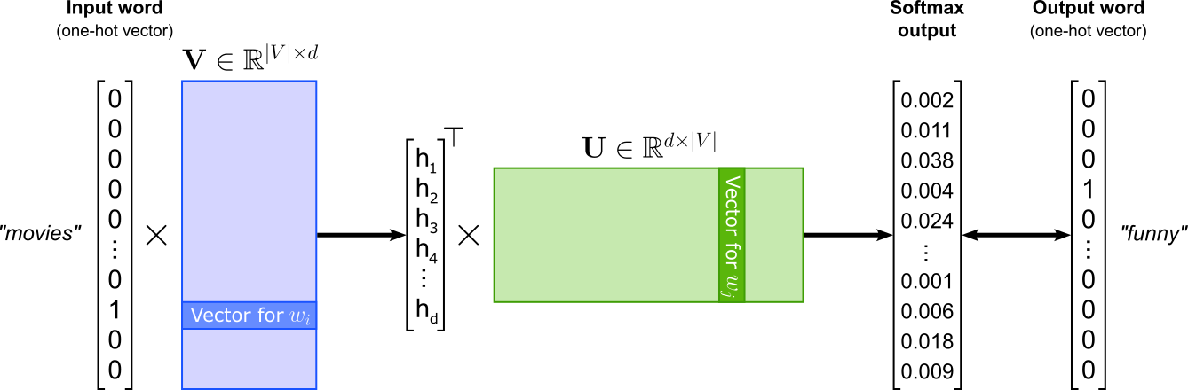
In its core, Word2Vec is implemented as a word classification task where the goal is to train a model that can predict word relationships based on their contexts. The figure below illustrates the general architecture assuming a single word as input and a single word as output. The Word2Vec model can be implemented as a shallow neural network contain one hidden layer — represented by input weight matrix $\mathbf{U}\in \mathbb{R}^{|V|\times d}$ — and one output layer — represented by input weight matrix $\mathbf{V}\in \mathbb{R}^{d\times |V|}$. Here, $V$ represents the vocabulary, i.e., the set of the unique words; naturally, $|V|$ is the size of the vocabulary, i.e., the number of unique words.
The embedding size $d$ is the dimensionality of the embedding vector used to represent each word, and it determines how much information the embedding can encode. A larger $d$ gives the model more capacity to capture nuanced semantic and syntactic relationships between words, potentially improving performance on downstream tasks — but it also increases the number of parameters, the risk of overfitting, and the computational cost. A smaller $d$ produces more compact embeddings that train faster and may generalize better on small datasets, but they might lack the expressive power needed to distinguish subtle word relationships. In practice, the optimal embedding size depends on dataset size, model complexity, and task requirements. Common pretrained Word2Vec models typically use embedding sizes of $100$, $200$, or $300$ dimensions, with $300$ being the most widely used configuration (e.g., the original Google News Word2Vec model). These values represent a practical balance: large enough to capture meaningful semantic structure, but small enough to train efficiently and avoid overfitting.
This classification setup is essential because it enables Word2Vec to learn semantic word embeddings indirectly through prediction. By training to correctly classify words in context, the model adjusts its internal word vectors, captured by $\mathbf{U}$ and $\mathbf{V}$ so that words appearing in similar contexts have similar representations. Thus, while Word2Vec's ultimate goal is not classification per se, framing it as such provides a simple and effective learning objective for capturing the statistical structure of language.
This basic setup for Word2Vec can be implemented in various ways. The three most common variants, the ones we cover in this notebook, are:
- Continuous Bag-of-Words (CBOW) predicts a target word based on its surrounding context words.
- Skip-gram predicts context words given a target word, learning to represent words that appear in similar contexts with similar vectors.
- Skip-gram with Negative Sampling (SGNS) is an optimized variant of Skip-gram that dramatically reduces training complexity by sampling a few negative examples instead of computing probabilities across the entire vocabulary.
It is arguably not obvious why this general setup of Word2Vec as a word prediction task will learn similar embedding vectors for words that are semantically similar (regarding the Distributional Hypothesis). However, this will become clearer when looking at the loss functions for the different variants and what minimizing those loss functions mean for the vectors in $\mathbf{U}$ and $\mathbf{V}$. In general, since Word2Vec learns a word prediction task, which itself is just a classification task, Word2Vec relies on the Cross-Entropy (CE) loss as the loss function to be be minimized:
where, given the figure above, $\hat{\mathbf{y}}$ is the softmax output and $\mathbf{y}$ is the one-hot vector representing the output or target word.
Continuous Bag-of-Words (CBOW)
In the Continuous Bag-of-Words (CBOW) setup of Word2Vec, the model predicts a target word (or center word) based on its surrounding context words. Given a window of text (for example, two words to the left and two to the right), CBOW averages or sums the embeddings of the context words and feeds this combined representation into a classifier that tries to guess the missing central word. Because the input is an unordered "bag" of context words, CBOW does not consider word order, which simplifies the model and speeds up training. For example, in the sentence "We were watching funny movies on Netflix last weekend", if the window size is $2$ and the target word is "movies", the context words would be "watching", "funny", "on", and "Netflix" (again, CBOW ignores the actual order).
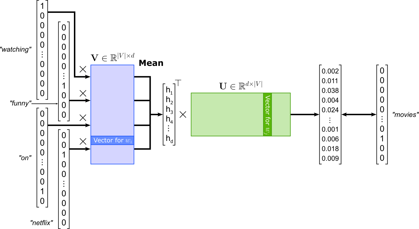
In practical terms, a single training sample contains the $2m$ context words and the center word to be predicted. For the example illustrated in the figure above, the training sample might look as follows — keep in mind that the order of the context words does not matter, even when shown as a list here:
(["watching", "funny", "on", "netflix"], "movies")
To better understand what the CBOW model is learning during training, let's have a look at the loss function. If you consider the Cross Entropy loss $\mathcal{L}_{\text{CE}}$ (see above), the only softmax output that matters is the one for the center word $w_c$; for all other words the target label in the one-hot vector is $0$. For CBOW, this softmax output reflects the probability of seeing the center word $w_c$ given the context words $w_{c-m}$, ..., $w_{c-1}$, $w_{c+1}$, ..., $w_{c+m}$, i.e.:
During training, we want to maximize this probability for each training sample. Since the consensus is that loss functions are minimized, we can simply consider the negative probability. Instead of raw probability, we also consider the log probability. This has the advantage that, when combining the losses of multiple samples, we can add log probabilities instead of multiplying raw probabilities. Thus, the loss function for a single training sample is:
Given the Word2Vec setup, the center word $w_c$ is represented by its corresponding embedding vector $\mathbf{u}_{c}$ in the output embedding matrix $\mathbf{U}$. Similarly, all $2m$ context words are represented by their embedding vectors $\mathbf{v}_{c-m}$, ..., $\mathbf{v}_{c-1}$, $\mathbf{v}_{c+1}$, ..., $\mathbf{v}_{c+m}$. Furthermore, since we treat the context words as a "bag" and ignore the sequence, CBOW represents all context words as a single embedding vector $\tilde{\mathbf{v}}$ as the mean of all context word embedding vectors. With this, we can write the loss as follows:
We also know that $P(\mathbf{u}_c\ |\ \tilde{\mathbf{v}})$ is computed using the softmax of the dot product between $\mathbf{u}_{c}$ and $\tilde{\mathbf{v}}$; more formally:
Now that we know how to compute the loss, we can actually see what is going to happen during training when trying to minimize the loss function $\mathcal{L}_{\text{CBOW}}$. Most obviously, we have minimized the loss when we have maximized the probability $P(\mathbf{u}_c\ |\ \tilde{\mathbf{v}})$. This probability, in turn, gets maximized if the value of dot product $\mathbf{u}_{c}^\top \tilde{\mathbf{v}}$ increases. Recall that a large dot product between two vectors means they are strongly aligned and have large magnitudes. Intuitively, this means one vector projects strongly onto the other: they share a strong directional similarity, one reinforces the other, and in applications such as embeddings this corresponds to high similarity.
By minimizing $\mathcal{L}_{\text{CBOW}}$, we force the embedding vectors between the center words and its context words to become more similar. Notice that this is not really what we are looking for. For example, we are not directly interested in the case where the embedding vectors for the words "movie" and "funny" are similar. However, this explicit training objective implies that (center) words that often appear in very similar contexts will also have similar embedding vectors. To see, this consider the phrase "watching funny videos on YouTube", with "videos" being the center words. Since (a) the words "movies" and "videos" often appear in (very) similar contexts, and (b) both their embedding vectors will be similar to embedding vectors of those shared context words, the embedding vectors for "movies" and "videos" will also be similar.
In terms of architecture, the CBOW model is a shallow neural network with one hidden layer. To give an example, the class CBOW in the code cell below is a straightforward implementation of the CBOW architecture as shown in the figure about using PyTorch. The model contains the implementations of the two weight matrices $\mathbf{U}$ and $\mathbf{V}$. Notice that the input weight matrix $\mathbf{U}$ is implemented using a nn.Embedding layer. This avoids the need to convert each word index into its respective one-hot vector. The class also performs the computation of the loss. The nn.CrossEntropyLoss is a commonly used loss function for multi-class classification tasks. It combines nn.LogSoftmax and nn.NLLLoss (negative log-likelihood loss) in a single step. Because nn.CrossEntropyLoss internally applies the log-softmax operation, the inputs to the loss function are raw scores (logits) rather than probabilities.
class CBOW(nn.Module):

    def __init__(self, vocab_size, embed_size):
        super(CBOW, self).__init__()
        self.embed_size = embed_size
        self.V = nn.Embedding(vocab_size, embed_size, max_norm=1)
        self.U = nn.Linear(embed_size, vocab_size)
        self.criterion = nn.CrossEntropyLoss()

    def forward(self, inputs, outputs):
        out = self.V(inputs)
        out = out.mean(axis=1)
        out = self.U(out)
        return self.criterion(out, outputs)
Using this model class, and a (preferably very large) dataset containing training samples in the format as shown above, we could now train our own CBOW Word2Vec embedding vectors. However, this is beyond the scope here, but we do have a dedicated notebook that goes through all required steps to train Word2Vec embeddings from scratch in great detail.
Skip-gram
The Skip-gram model of Word2Vec is the "opposite" of the CBOW model: Instead of predicting the center or target word given the context words like in CBOW, Skip-gram is modeled to predict the context words given the center words. Using the same example, given the word "movies", Skip-gram learns to predict the context words "watching", "funny", "on", and "netflix". Again, the order of the context words does not matter. The model architecture of SKip-gram is very similar to CBOW; see the figure below. Since Skip-gram takes in a single word, there is no longer a need to compute the average of multiple inputs embeddings. In contrast, Skip-gram has to compute multiple losses with respect to each predicted context word.
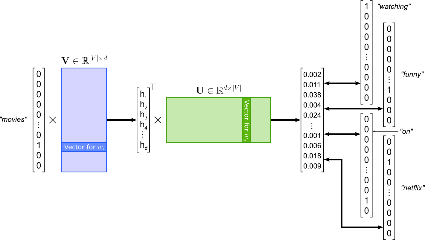
Since the losses between a center word and all context words are independent from each other, we can treat each (center, context) pair as its own training samples. This means, given the example illustrated in the figure above with a window size of $2$, we get the following $4$ training samples:
("movies", "watching")
("movies", "funny")
("movies", "on")
("movies", "netflix")
Like for the CBOW model, let's have a closer look at the loss for Skip-gram. Naturally, the mirrored nature of both models is also reflected by their losses. This means that for a single training sample the output of the model reflects the probability of seeing the context words $w_{c-m}$, ..., $w_{c-1}$, $w_{c+1}$, ..., $w_{c+m}$ given the context word $w_c$:
Again, negating the probability to get a proper loss function and computing the log probabilities for mathematical convenience, we get the following basic formulation for the Skip-gram loss $\mathcal{L}_{\text{Skip-gram}}$:
Since the context words are treated as a bag of words and only their presence matters but not their order, the probability of seeing a context word given center word $w_c$ does not depend on the other context words. Due due to this independence, we can rewrite the loss function as follows — appreciate how the use of log probabilities comes in handy now:
Representing the context words and the center word once more with their corresponding embedding vectors — now the center words is taken from input embedding matrix $\mathbf{V}$ and the context words are taken from output embedding matrix $\mathbf{U}$, we get the final definition of the Skip-gram loss:
The individual probabilities $P(\mathbf{u}_{c+j} | \ \mathbf{v}_c)$ are again simply the softmax output of the dot products. More specifically, in the case of Skip-gram (compared to CBOW) these softmax outputs are computed as:
In crude terms, the softmax outputs of both CBOW and Skip-gram result from the dot products between "some input embedding and some output embedding vectors" where the pairing depends on words' contexts. This also means that Skip-gram minimizes its loss $\mathcal{L}_{\text{Skip-gram}}$ when the corresponding embedding vectors of center words and their context words become more and more similar, which means that two (center) words with often similar context will yield embedding vectors that are similar — and thus implementing the idea of the Distributional Hypothesis.
The implementation of the Skip-gram model is equally straightforward as for the CBOW model; the code cell below shows the most basic implementation in PyTorch. The main difference compared to the CBOW class above is that the forward() method no longer computes any means of input embedding vectors. This, of course, assumes that the training samples have the format as shown above, i.e., (center, context) word pairs.
class Skipgram(nn.Module):

    def __init__(self, vocab_size, embed_size):
        super(Skipgram, self).__init__()
        self.embed_size = embed_size
        self.V = nn.Embedding(vocab_size, embed_size, max_norm=1)
        self.U = nn.Linear(embed_size, vocab_size)
        self.criterion = nn.CrossEntropyLoss()

    def forward(self, inputs, outputs):
        out = self.V(inputs)
        out = self.U(out)
        return self.criterion(out, outputs)
CBOW vs. Skip-gram. Despite their close relationship, in practice, CBOW and Skip-gram tend to produce slightly different types of word embeddings, but most of the differences are empirical observations rather than strict theoretical guarantees. CBOW predicts a target word from its surrounding context, which effectively averages the context information. Because of this averaging, CBOW is faster to train, more stable, and works better on large datasets, especially for learning good representations of frequent words. In contrast, Skip-gram predicts the surrounding words from a target word, which means it sees many more training examples for each word. This makes Skip-gram slower but tends to yield better representations for rare words, because every training instance focuses on a single central word instead of a blurred context window; it is also better at capturing fine-grained semantic relationships. To summarize the empirical differences:
- CBOW performs better when the dataset is very large, and you want fast, stable training and good embeddings for common words.
- Skip-gram performs better when the dataset is small or medium-sized, or when rare words matter, because it learns richer embeddings for infrequent terms.
Skip-gram with Negative Sampling (SGNS)
The basic Skip-gram model tries to predict every context word in a window using a full softmax over the entire vocabulary. While conceptually simple, this is computationally expensive because each training step requires computing scores for all vocabulary items, which can easily be millions of words. This makes vanilla Skip-gram impractical for large corpora and leads to very slow training. Moreover, many of the predicted context words are actually uninformative for learning meaningful embeddings, since most words in the vocabulary are not relevant exceptions for any given training example. For example, determiners ("a", "an"), conjunctions ("and", "or", "but", etc.), or prepositions ("to", "from", "up", etc.) are words that appear in the contexts of basically all words.
Skip-gram with Negative Sampling (SGNS) addresses these issues by replacing the full softmax with a binary classification task: the model learns to distinguish real context words from a small number of artificially sampled "negative" words (i.e., negative samples). Instead of comparing the target word to the entire vocabulary, SGNS compares it only to a handful of negative samples, making each update dramatically faster. This allows training on huge datasets while still pushing embeddings of related words closer and unrelated words further apart. Thus, for our example center word and corresponding context words, the positive samples together with "some" negative sample would look conceptually as follows:
(["movies", "watching"], 1)
(["movies", "funny"], 1)
(["movies", "on"], 1),
(["movies", "netflix"], 1)
(["movies", "tall"], 0)
(["movies", "from"], 0)
(["movies", "elephant"]), 0),
(["movies", "because"], 0)
(["movies", "train"], 0)
(["movies", "delicious"], 0)
(["movies", "separate"], 0),
(["movies", "still"], 0)
Here, the true or positive samples (i.e., the samples representing true pairs of center and context words) are labeled with $1$. The samples labeled with $0$ are the negative samples and are pairs of center words and other words that are (generally) not context words of the center word. In general, negative samples are generated randomly by selecting words from the vocabulary and pairing them with a given center word. While a random word might be a context word of the center word somewhere in the corpus, the probability is negligible (assuming a sufficiently large vocabulary). However, the random sampling is tweaked to favor the selection of rare words (discussed later).
This simplified setup as a binary classification task is also reflected by the loss function. In principle, we could directly use the idea of an annotated datasets (with the two labels $O$ and $1$) and compute the Cross Entropy loss during training. However, there is a smarter and more efficient way to compute the loss. To see how this works, we first need to acknowledge that we now want to maximize two probabilities depending on whether the sample is a positive sample or a negative sample. More formally, we want to maximize
- $P(+|\ c,m)$ if the (center, context) word pair $(c,m)$ is in the batch of positive samples $B_{pos}$, and
- $P(-|\ c,m)$ if the (center, context) word pair $(c,m)$ is in the batch of negative samples $B_{neg}$
Combined with the independence between all context words, we can express the loss function as the product of all probabilities $P(+|\ c,m)$ and $P(-|\ c,m)$, including the application of the logarithm and negating the result, giving us:
Since we have binary classification task, we know that $P(+|\ c,m) + P(-|\ c,m) = 1$, as well as $P(-|\ c,m) = 1 P(+|\ c,m)$. We can therefore rewrite the previous expression as:
We can further simplify the expression by converting the logarithm of a product of probabilities to a sum of log probabilities by applying common logarithm rules:
Computing $P(+|\ c,m)$ is not much simpler compared to CBOW and Skip-gram due to having a binary classification task because instead of the softmax we only need to compute the sigmoid function for the dot product between the corresponding input and output embedding vectors for the center and context words. If we do this, we get the following:
For the last simplification step, consider the following sequence of equations where we can get rid of the "$1-$" in front of the sigmoid function.
Applying this step to our loss function, we get:
The only remaining rewrite we can do is simply to replace the full expression of the sigmoid function with the commonly used function name $\sigma$ — but this is merely to make reading and writing the loss function more convenient.
Compared to the Cross Entropy loss, this $\mathcal{L}_{\text{SGNS}}$ is not a standard loss function implemented in libraries such as PyTorch. However, we can easily implement this loss function in PyTorch; the code cell below shows an example implementation. In this code, u_pos represents all context word embeddings in the positive samples, and u_neg all context word embeddings in the negative samples. The rest of the forward method directly implements the formula for $L_{SGNS}$ as shown above.
class NegativeSamplingLoss(nn.Module):

    def __init__(self):
        super().__init__()

    def forward(self, v_c, u_pos, u_neg):
        # Computes positive scores and losses
        pos_score = torch.bmm(u_pos.unsqueeze(1), v_c.unsqueeze(2)).squeeze()
        pos_loss = F.logsigmoid(pos_score)
        #  Compute negative scores and losses
        neg_score = torch.bmm(u_neg, v_c.unsqueeze(2)).squeeze()
        neg_loss = F.logsigmoid(-neg_score).sum(1)
        # Return total loss (negative log-likelihood)
        return -(pos_loss + neg_loss).mean()
In PyTorch, torch.bmm() (batch matrix–matrix multiplication) performs matrix multiplication on an entire batch of matrices at once. Instead of multiplying two matrices of shape $(m \times n)$ and $(n \times p)$, bmm() multiplies two tensors of shape $(B \times m \times n)$ and $(B \times n \times p)$, producing a result of shape $(B \times m \times p)$ — where $B$ is the batch size. This makes it ideal for models that must process many independent matrix multiplications in parallel such as working with multiple samples simultaneously. The complete implementation of the SGNS model is a bit more complicated compared to CBOW and vanilla Skip-Gram, so we do not show an example implementation here. However, you can find all the implementation details in the notebook training Word2Vec embedding vectors for all three Word2Vec variants from scratch.
Sampling strategies. In SGNS, smoothing is applied when selecting negative samples to ensure a balanced mix of common and rare words. In the raw corpus, words follow a very skewed Zipfian distribution: a few words occur extremely often while most occur rarely. If negative samples were drawn strictly according to this distribution, the model would overwhelmingly see common words like "the", "and", or "is" as negatives., Thus, instead of sampling negatives directly from the raw unigram distribution $U(w)$, the model samples from a smoothed distribution defined as:
where $U(w)$ is the unigram probability of word $w$ (its frequency divided by the total number of tokens), the exponent $3/4$ is a smoothing factor chosen empirically, and $Z = \sum_{w'} U(w')^{3/4}$ is a normalization constant ensuring $P(w)$ sums to 1. This smoothing reduces the probability of sampling very frequent words and increases the chance of sampling less frequent ones as negative examples. As a result, the negative samples are more informative and diverse, helping the model learn better embeddings.
Basic Properties
Word2Vec embeddings provide compact, efficient representations by mapping each word to a low-dimensional dense vector instead of a sparse, high-dimensional one-hot encoding. This makes them inexpensive to store and fast to use while still capturing rich linguistic information. Because information is distributed across dimensions, embeddings can generalize smoothly: words that appear in similar contexts end up with similar vectors, even if they rarely co-occur directly. They are also robust to noise and variability in language use. By aggregating contextual evidence across many occurrences, Word2Vec forms stable, context-invariant representations that reflect the dominant meaning of a word rather than idiosyncratic or rare usages. This smoothness and robustness make the embeddings practical and reliable inputs for a wide range of NLP tasks.
Vector Similarities
The main goal of word embedding methods such as Word2Vec is to learn embedding vectors that map words with similar meaning to similar vectors. To illustrate this, the plot below shows some example results using CBOW — in fact, this plot is generated as part of the notebook where you can train Word2Vec word embeddings from scratch. In a nutshell, this notebook uses a small dataset of $100,000$ movie reviews and the CBOW model to learn the embedding vectors for the $10,000$ most frequent words. The learned vectors have a size of $100$ dimensions.
The plot shows the $5$ most similar words for a set of seed words (see the legend in the plot) based on similarities between their respective embedding vectors using the cosine similarity. To plot the $100$-dimensional vectors, we use the dimension reduction technique t-SNE to map the embedding vectors from the $100$-dimensional space to a $2$-dimensional space.
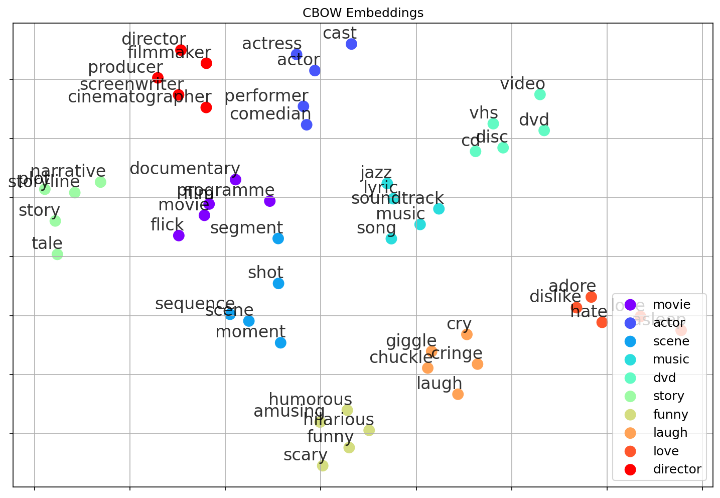
Overall, the results show that words with similar meaning are indeed now represented using similar vectors; each seed word together with its $5$ most similar words (which includes the seed word itself) form a rather tight cluster (reflected by points of the same color in the plot). However, when looking more closely at some of the words considered most similar, you may notice some cases that are arguably less intuitive. We will later come back to this when talking about basic limitations of Word2Vec (and similar approaches).
Linear Subspaces — Analogies
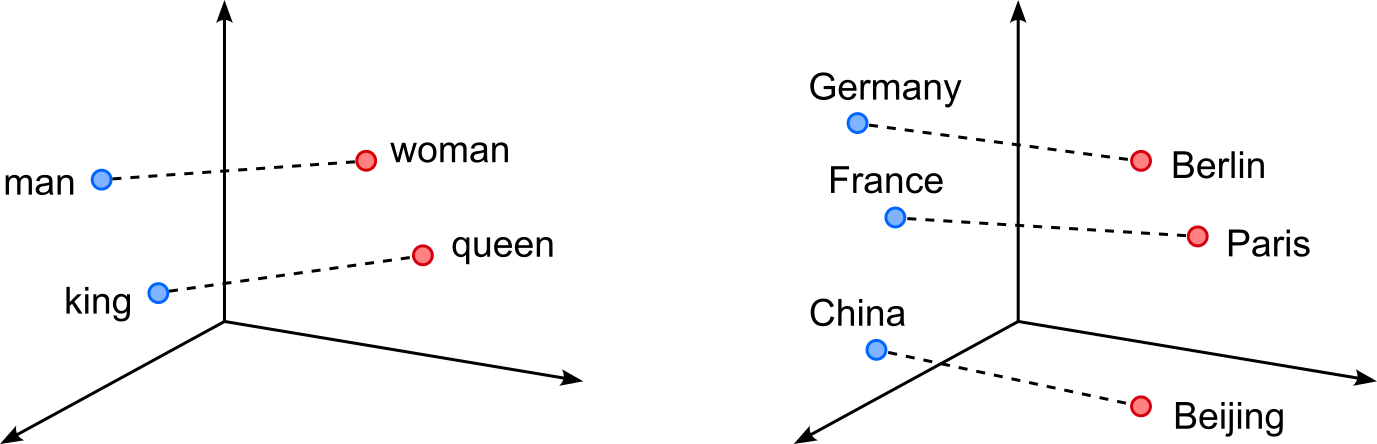
That two words that are semantically similar get represented by learned embedding vectors that are similar in the embedding space is kind of the "minimum" desired property of Word2Vec and related embedding methods in general. However, another striking empirical property of Word2Vec embeddings is that certain semantic or syntactic relations correspond to approximately linear directions in the embedding space. This means that words participating in the same type of relation (e.g., gender, verb tense, plurality, country–capital) tend to differ by similar displacement vectors.
For example, in the figure (right) below, the vector difference $king − man$ is often close to $queen − woman$, which allows analogies to be solved by simple vector arithmetic such as $king − man + woman \approx queen$. Rather than being isolated coincidences, these relations can be understood as lying in low-dimensional linear subspaces spanned by a small number of such relation-specific directions. The left figure shows similar analogies using the relation between countries as capitals as an example. Here the vector difference $Germany - Berlin$, $France - Paris$, and $China - Beijing$ are likely to be very similar. This again allows for meaningful arithmetic operations such as $France - Paris + Berlin \approx Germany$.
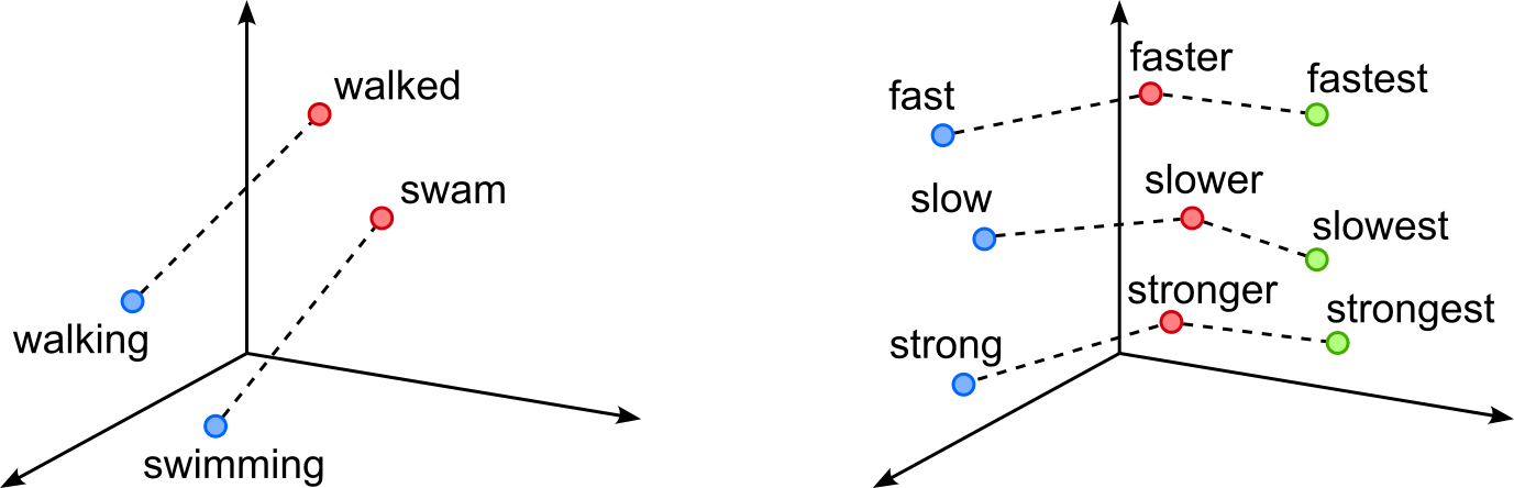
These kinds of relations in low-dimensional subspaces are not limited to nouns and proper nouns. The figure below shows similar examples for verbs with respect to differences in tenses (left figure), and for adjectives with respect to their base form, comparative, and superlative.
The underlying intuition is that Word2Vec is trained to preserve patterns of word co-occurrence: words that appear in similar contexts are close together, and systematic contextual differences induce consistent offsets. When a semantic attribute (like gender or tense) affects word usage in a regular way across many word pairs, the model can encode this attribute as a roughly linear factor in the embedding space. As a result, analogical reasoning reduces to linear algebra, and entire families of analogies can be captured by projecting word vectors onto the corresponding subspace. This linear structure is not explicitly enforced during training, but emerges naturally from the objective and the distributional regularities of language.
The existence of linear subspaces and consistent relation vectors in Word2Vec embeddings indicates that the individual dimensions are not arbitrary, but jointly organize semantic information in a structured way. Although no single dimension corresponds directly to an interpretable concept like "gender" or "tense" these concepts are nonetheless encoded as directions or combinations of dimensions. If the dimensions were purely meaningless or random, we would not observe stable, reusable displacement vectors such as $king − man \approx queen − woman$ across many word pairs. The fact that such relations generalize implies that semantic attributes are distributed across dimensions and can be recovered through linear operations, revealing that the embedding space has a coherent internal geometry shaped by meaning.
This phenomenon reflects the idea of distributed representations: semantics is encoded in patterns across many dimensions rather than in isolated coordinates. Each dimension may contribute weakly to multiple semantic factors, but together they form subspaces that correspond to meaningful linguistic properties. As a result, while individual axes lack an intuitive 1:1 interpretation, the embedding as a whole supports semantically meaningful computations like analogy solving, clustering, and similarity measurement. The emergence of linear structure therefore provides strong evidence that word embeddings capture latent semantic factors, even when these factors are only interpretable at the level of vector combinations rather than single dimensions.
Important: Despite their appeal, linear subspaces and vector arithmetic in Word2Vec are only approximate phenomena rather than strict algebraic rules. Many analogies work well, but a substantial number fail or produce unstable results depending on the vocabulary, training data, embedding dimension, or similarity metric used. Even for commonly cited relations like gender or tense, the corresponding direction is often noisy and entangled with other semantic factors. As a result, operations such as $a − b + c$ do not reliably yield the expected word $d$, and small changes in the input words or model can lead to different or less interpretable outcomes. These observations suggest that analogy-solving via vector arithmetic should be seen as an emergent statistical regularity, not as a precise compositional mechanism. Language is highly polysemous and context-dependent, and many relations between words are not uniform across all instances or domains. Consequently, semantic relations may not lie in clean, low-dimensional subspaces, but instead overlap and interfere with one another. The success of linear analogies therefore highlights useful structure in embedding spaces, while their frequent failures remind us that this structure is imperfect and that word embeddings provide an approximate, distribution-driven representation of meaning rather than a complete semantic model.
Practical Considerations & Limitations
While Word2Vec and similar embedding approaches have become fundamental tools in NLP, their practical use requires careful consideration of their limitations. These models learn word meaning purely from co-occurrence statistics, which means their quality depends heavily on factors such as corpus size, domain, vocabulary frequency, and training hyperparameters. As a result, seemingly small choices like window size or negative sampling rates, can significantly influence the semantic structure of the learned space.
Moreover, these methods inherit several intrinsic constraints: they produce a single vector per word type (ignoring polysemy), are sensitive to biases present in the training data, and may struggle with rare or unseen words. Understanding these practical considerations and limitations is essential for using Word2Vec effectively, evaluating its outputs correctly, and deciding when more advanced embedding techniques may be necessary. Let's look at some of those considerations and limitations a bit more closely.
Effects of Training Data
When training Word2Vec or any other word embedding model, the choice of the training dataset is crucial because word meaning is learned entirely from the contexts in which words appear. These models have no built-in understanding of language; instead, they infer semantic and syntactic relationships by observing which words tend to co-occur. If the dataset is biased toward specific topics, writing styles, or domains, the learned embeddings will reflect those patterns. For example, embeddings trained on biomedical texts will capture technical, domain-specific relationships that differ substantially from embeddings trained on news articles, literature, or social media.
To give a concrete example, the table below shows the top-10 most similar words to the word "house" with respect to their corresponding learning embedding vectors. The two rankings refer to two pretrained sets of word embedding using different datasets. One was trained on a large dump of Wikipedia articles, while the other was trained on a large Google News dataset. Overall both rankings look good since all listed words are indeed semantically similar to "house". However, there are differences in the rankings. Most prominently, the ranking for Wikipedia contains arguably main old-timey or less modern words such as "cottage" or "parsonage" which are missing from the Google News ranking (which mostly contains "modern" words).
| Rank | Wikipedia | Google News |
|---|---|---|
| 1 | mansion | houses |
| 2 | cottage | bungalow |
| 3 | farmhouse | apartment |
| 4 | barn | bedroom |
| 5 | bungalow | townhouse |
| 6 | townhouse | residence |
| 7 | houses | mansion |
| 8 | parsonage | farmhouse |
| 9 | tavern | duplex |
| 10 | summerhouse | apprtment |
The choice of dataset matters because the usefulness of word embeddings depends on how well the training data matches the target task. For general-purpose embeddings, the goal is to capture broad semantic and syntactic patterns that hold across many domains. This requires a very large and diverse corpus that spans different topics, writing styles, and genres. Such variety helps the model learn stable, domain-agnostic representations and reduces the risk of overfitting to niche vocabulary or stylistic quirks. It also mitigates unwanted biases by exposing the model to a wider range of language use rather than letting any single domain dominate.
In contrast, for domain-specific tasks such as medical text mining, legal document analysis, or analyzing social media language, the ideal training dataset should closely resemble the text the embeddings will be applied to. This ensures that the model captures the specialized terminology, context patterns, and linguistic conventions relevant to that domain. A mismatch between training data and target task can lead to poor performance, because the embeddings may represent words in ways that are irrelevant, or even misleading, for the intended application. Thus, choosing the right dataset is essential for producing effective and reliable word embeddings.
Preprocessing Steps
Preprocessing choices significantly influence the quality and behavior of word embeddings because they determine what the model sees as a "word", how consistently tokens appear, and what linguistic distinctions are preserved. When preparing a raw text corpus to serve as a training dataset for a word embedding model, there are various design decisions you have to make that will affect the resulting embeddings. Here are some of the most relevant considerations
Choice of tokenizer. The tokenizer governs how text is split into units; simple whitespace tokenizers may merge punctuation with words or mishandle compound terms, while more sophisticated tokenizers can better capture linguistic structure. For tasks involving noisy text (e.g., social media), tokenizers that handle emojis, URLs, or slang may yield more informative embeddings.
Case-folding. The conversion of a that all lowercase letters/characters reduces sparsity by merging variants like "Apple" and "apple", but it also removes distinctions that may matter in specific domains such as named-entity-heavy corpora (news, biomedical, legal). For example, converting the company name "Apple" to lowercase makes indistinguishable from the fruit.
Stemming or lemmatization. Similar case-folding, stemming and lemmatization also reduces sparsity, but here by reducing inflectional forms to a base form (e.g., "houses"$\rightarrow$"house", "went"$\rightarrow$"go", "faster"$\rightarrow$"fast"), which can help when the focus is on capturing general semantic relationships rather than fine-grained grammatical nuances. However, this also removes morphological information that might be useful, especially in morphologically rich languages or tasks where verb tense and number matter.
Stopword removal. Removing high-frequency, low-information words such as determiners, conjunctions, or prepositions can sometimes help downstream tasks but is often discouraged for embedding training. Word2Vec relies on natural co-occurrence statistics, and removing stopwords can distort sentence structure and eliminate valuable syntactic signals — so many practitioners keep them.
Cross-sentence context. When determining the context of a (center) word, you can decide whether to consider only words within sentence boundaries or across them. Limiting training to within-sentence contexts usually produces cleaner syntactic relationships and avoids linking words that appear near each other only due to formatting or layout. But for certain tasks (e.g., document classification or discourse modeling) allowing cross-sentence windows can capture broader topical associations.
Summing up, preprocessing decisions depend heavily on the dataset's characteristics (formal vs. informal, domain-specific vocabulary, noise level) and the downstream task (semantic similarity, classification, named entity tasks, etc.). The key is to balance reducing noise and sparsity while preserving the linguistic signals that are meaningful for your application.
Choice of Hyperparameters
One of the most important hyperparameters when training Word2Vec embeddings is the context window size $m$, which determines how many words before and after a target word are used during training. The window size directly controls what type of semantic information the model captures:
- Smaller windows (e.g., $2\!-\!5$ words) focus on very local context, emphasizing syntactic relationships such as part-of-speech patterns or short-range dependencies (e.g., "eat $\rightarrow$ food", "run $\rightarrow$ quickly"). These windows encourage embeddings that encode functional similarity.
- Larger windows (e.g., $8\!-\!15$ words) capture broader topical or semantic relationships, yielding embeddings where words appearing in the same theme or discourse (e.g., "hospital", "doctor", and "treatment") cluster together even if they do not co-occur closely.
In short, context size balances fine-grained syntactic information versus coarse semantic associations. In practice, common window sizes range from $2$ to $5$ for syntax-sensitive tasks to $5$ to $10$ (or even $15$) for semantic similarity or topic-related tasks. The typical default in many implementations (including the original Word2Vec code) is around $5$. While both CBOW and Skip-gram use window size in similar ways, there are subtle practical differences: CBOW tends to perform well with slightly larger windows because it aggregates multiple context words to predict the target, making it robust to noisier or broader contexts. Skip-gram, which predicts each context word individually, often benefits from smaller or moderate windows, as large windows dramatically increase the number of training pairs and may introduce more noise. Ultimately, choosing the right window size depends on the task: narrow windows for syntactic tasks, wider windows for semantic or domain-specific concept learning.
In the case Skip-gram with Negative Sampling (SGNS), there is also number of negative samples as a hyperparameter. It controls how strongly the model learns to distinguish true word-context pairs from randomly sampled, "incorrect" ones. Each negative sample forces the model to push apart embeddings of words that do not co-occur, so using more negative samples generally sharpens the model's ability to separate meaningful relationships from noise. With too few negative samples, the model may not learn enough contrast, leading to weaker or blurrier embeddings. With too many, training becomes slower and may overemphasize rejecting unlikely contexts, which can add noise or reduce the subtlety of learned semantic relations.
In practice, the optimal number of negative samples depends on corpus size and vocabulary frequency distribution, but typical values are small. Mikolov et al. (the original Word2Vec authors) recommend $5$ to $20$ negative samples per positive pair, with $5$ to $10$ being common defaults. For large datasets, even fewer negatives (e.g., $2$ to $5$) often work well because the sheer volume of training examples compensates for the smaller contrast signal. Conversely, for smaller or noisier datasets, using more negative samples can help stabilize training and improve embedding quality. Overall, the number of negatives balances computational cost and the strength of the contrastive signal, and modest values tend to perform well across a wide range of tasks.
Unmodeled Semantics
The Distributional Hypothesis — that is, the idea that two words are similar if they are often used in similar contexts — is a powerful and intuitive concept. However, it is not powerful enough to capture aspects of a word's meaning. To give an example, look at the plot showing the example embeddings from before, only with some word clusters highlighted. Some of the words that are considered similar according to Word2Vec might actually seem to be rather opposite. For example, "adore" and "hate" are close together, and so are "laugh" and "cry", as well as "funny" and "scary".
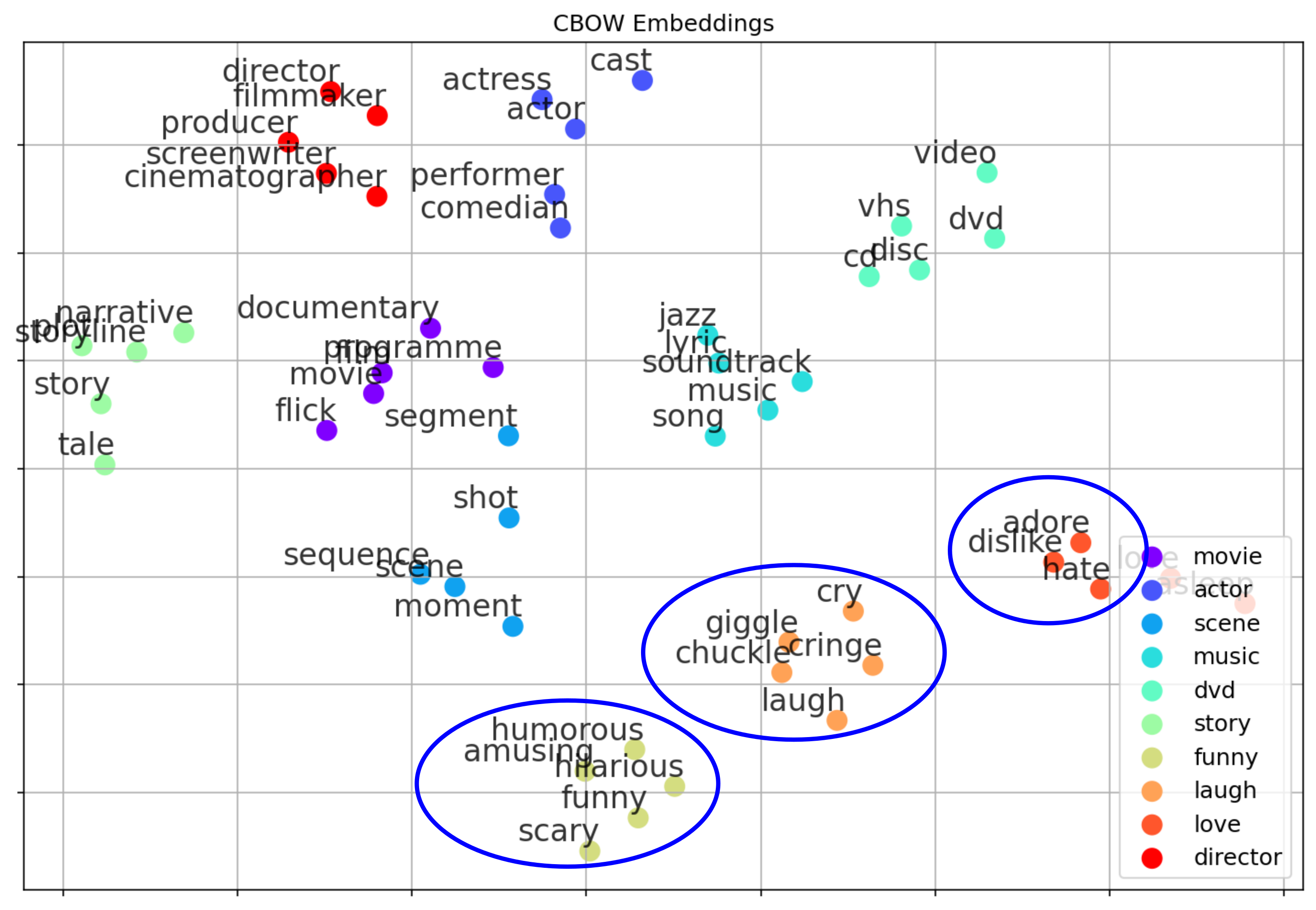
While these results do not seem intuitive, they do match the idea of the Distributional Hypothesis. For example, "adore" and "hate" are used to express a sentiment, opinion, or feeling towards someone or something — only with a different polarity. As such, both words are likely to appear in similar contexts and therefore yield similar vector representations. This is a concrete case showcasing that the Distributional Hypothesis does not capture all possible facets of a word's meaning. Here it clearly indicates that it is unable to capture words' polarity. Such insights are important, for example, when training models for sentiment classification based on pretrained Word2Vec word embeddings.
One Word = One Vector
Word2Vec and similar early embedding methods learn one fixed vector per word, regardless of how many meanings or grammatical roles that word may have. This means that polysemous words such as "bank", "apple", or "run" are forced into a single representation even though they appear in very different contexts. As a result, the embedding becomes an average of all the word's usages, blending together meanings that should ideally be kept separate. This averaging can blur distinctions and reduce the usefulness of the embeddings for tasks that rely on precise semantic understanding. To give an example, consider the following sentence:
A light wind will make the traffic light collapse and light up in flames
Just by looking at the three occurrences of the word "light", we can see the issue that arises when encoding the same word using the same embedding vector. For one, all three occurrences of "light" serve a different syntactic function: first an adjective, then a noun, and lastly a verb. But even even with respect to the same syntactic function, the same word may have (very) different meanings. For example, a traffic light is arguably a very different thing compared to a torch light — or just the noun "light" in a sentence like "I saw the light at the end of the tunnel". In short, using the same embedding vector for "light" fails to capture the word's syntactic function and proper meaning. This is where attention comes in.
This is a clear limitation because many downstream NLP applications (e.g., word sense disambiguation, semantic search, parsing, or contextual language understanding) require distinguishing between different senses or functions of the same word. A static embedding cannot adapt to context: the same vector is used whether "bank" refers to a financial institution or the side of a river. This restricts the model's ability to represent nuances and can lead to poorer performance compared to modern contextual embeddings (e.g., from BERT or GPT), which dynamically adjust word representations based on surrounding text.
Summary
This notebook introduced the Word2Vec family of models, focusing on its three main variants: Continuous Bag-of-Words (CBOW), Skip-gram, and Skip-gram with Negative Sampling (SGNS). CBOW predicts a target word based on its surrounding context, making it computationally efficient and effective for large datasets. Skip-gram does the reverse, predicting context words from a target word, which is particularly useful for capturing rare words. SGNS refines Skip-gram by replacing the expensive full softmax with negative sampling, dramatically improving training speed while preserving high-quality embeddings. Together, these models form the foundation of early dense word vector representations.
A central insight of Word2Vec is that the learned embeddings encode meaningful geometric structure. Words with similar meanings cluster together, and specific linguistic relationships correspond to approximately linear subspaces within the vector space. Classic examples include analogies like $king – man + woman \approx queen$, reflecting how the model captures semantic and syntactic patterns purely from co-occurrence statistics. These properties made Word2Vec a breakthrough for many NLP tasks and helped shift the field toward distributed representations.
The notebook also discussed several practical considerations when training Word2Vec. Hyperparameters such as context window size, vector dimensionality, and the number of negative samples strongly influence the type of relationships the model captures. Preprocessing choices, including tokenization, case-folding, stopword handling, or stemming, shape what counts as a “word” and how often it appears. Dataset selection is equally important: embeddings trained on general-purpose corpora behave differently from those trained on specialized domains. Understanding these factors is essential to produce robust, meaningful word vectors.
Despite its strengths, Word2Vec comes with notable limitations. The model assigns a single static vector to each word type, even though many words are polysemous or function differently depending on context. This inability to represent meaning dynamically can blur important distinctions and limit performance in applications requiring fine-grained semantic understanding. Additionally, Word2Vec cannot naturally handle out-of-vocabulary words and struggles with morphological variability unless paired with subword models.
For these reasons, static embeddings like Word2Vec, GloVe, or FastText have largely been superseded by contextual embeddings from modern transformer-based models such as BERT, RoBERTa, and GPT. These newer models generate representations that adapt to each occurrence of a word, capturing its meaning in context and handling polysemy, syntax, and morphology far more effectively. Word2Vec remains historically important and conceptually elegant, but dynamic embeddings have become the dominant paradigm in contemporary NLP.