Disclaimer: This Jupyter Notebook contains content generated with the assistance of AI. While every effort has been made to review and validate the outputs, users should independently verify critical information before relying on it. The SELENE notebook repository is constantly evolving. We recommend downloading or pulling the latest version of this notebook from Github.
Word & Text Embeddings — An Overview
Word and text embeddings are numerical vector representations of linguistic units such as words, sentences, or entire documents, that are designed to capture semantic and syntactic properties of language. Instead of treating words as discrete symbols (e.g., IDs or one-hot vectors), embeddings map them into a continuous vector space where similar words or texts are located close to one another. This geometric structure allows models to reason about meaning using simple mathematical operations such as dot products or cosine similarity. In practice, embeddings form the backbone of most modern NLP systems, enabling tasks such as information retrieval, text classification, sentiment analysis, question answering, and recommendation systems to operate effectively and at scale.
The practical importance of embeddings stems from their ability to generalize beyond exact word matches. Because embeddings encode semantic similarity, models can recognize that words like "car" and "automobile" or texts discussing the same topic are related, even if they do not share identical tokens. This greatly improves robustness to vocabulary variation, synonymy, and noise. Moreover, embeddings provide a compact and dense representation of language, reducing the dimensionality and sparsity issues associated with traditional representations such as one-hot encoding or Bag-of-Words, and making them well-suited as inputs to neural network-based models.
In this notebook, we first motivate the importance and relevance of word and text embeddings, as well as the core linguistic idea behind most approaches to automatically generate or learn good embeddings: the Distributional Hypothesis. The main part of the notebooks then provides an overview to various foundational and popular word and text embedding methods in a systematic manner by organizing the overview along fundamental characteristics of embedding methods. The main learning outcomes are understanding the challenges when working with textual data and machine learning algorithms (particularly neural networks), as well as understanding and comparing different embedding strategies on a high level. Let's get started.
Setting up the Notebook
As the purpose of this notebook is to provide a general overview to concepts and solutions for finding good word and text embeddings, there so no code and therefore no libraries need to be imported.
Preliminaries
Before checking out this notebook, please consider the following:
This notebooks does not feature complete list of word and text embedding methods. Given the importance of embeddings, this is a very active field of research. In this notebook, we therefore focus on foundational and popular methods, and from a wide range of general strategies. This includes more "traditional" methods to highlight initial approaches but also their common limitations.
Modern embedding methods rely on neural network architectures such as Recurrent Neural Networks (RNNs) or Transformers. Although not fundamentally required here, some basic knowledge about these architecture is recommended to better appreciate relevant embedding methods.
Motivation
Why do we Need (Good) Embeddings?
Textual data is considered unstructured because, it does not follow a predefined format that explicitly encodes meaning. Natural language is highly variable: the same idea can be expressed in many different ways, words are ambiguous and context-dependent, and structure such as syntax or semantics is implicit rather than explicitly labeled. The inherent complexity of language is a key reason why neural network models have become the dominant approach for solving NLP and related tasks. Traditional rule-based or linear models struggle to capture these nonlinear and hierarchical patterns, as linguistic phenomena often depend on subtle interactions between words, syntax, and broader context. Neural networks, in contrast, can learn rich, high-dimensional representations directly from data and model complex relationships through layered transformations and distributed representations.
However, when it comes to using neural networks for NLP and related tasks, text is in fact a rather "inconvenient" for of data to work with, for the following to main reasons:
Variable sequences vs. fixed-sized inputs: Text, generally speaking, can be considered as a sequence of words (more generally: tokens) of variable length. Neural network models, on the other hand, assume standardized or canonical inputs, which typically entails inputs of a fixed size. Even sequence models such as Recurrent Neural Networks (RNNs) that can handle sequences of variable lengths, still require that the input at each time step is if a fixed size — of course, also words are just sequences of letters of variable size.
Nominal/symbolic data vs. numerical inputs: From a data perspective, words/tokens are just nominal or symbolic data, i.e., data that consists of discrete labels or categories without any inherent numerical meaning or ordering. That fact the words such as "cat" and "kitty" might be similar because words are labels for real-world concepts, and these concepts are similar in our mental model of the world. To a machine, "cat" and "kitty" are completely different strings. In contrast, neural network models fundamentally rely on numerical input because their learning and inference processes are defined by mathematical operations such as matrix multiplications, additions, nonlinear transformations, and optimization via gradient-based methods. These computations require inputs to lie in a continuous or at least ordered numerical space where notions like magnitude, similarity, scaling, and distance are well defined.
The illustration below summarizes these challenges. Presumably, if you would hear or read the sentence "I saw a cat" or "I saw a kitty", you picture more or less the same situation since a "kitty" is commonly used to refer to a small/young cat. When we hear or read a word, we typically do not process it as an abstract symbol in isolation but instead associate it with a mental representation of the real-world concept it refers to. This can include visual imagery, sensory impressions, experiences, or related ideas that have been learned through interaction with the world. Such mental associations allow us to grasp meaning quickly, reason about context, and connect language to prior knowledge, which is why words can evoke rich and nuanced understanding far beyond their written or spoken form alone. In short, to us, the two words and therefore the two sentences are similar.
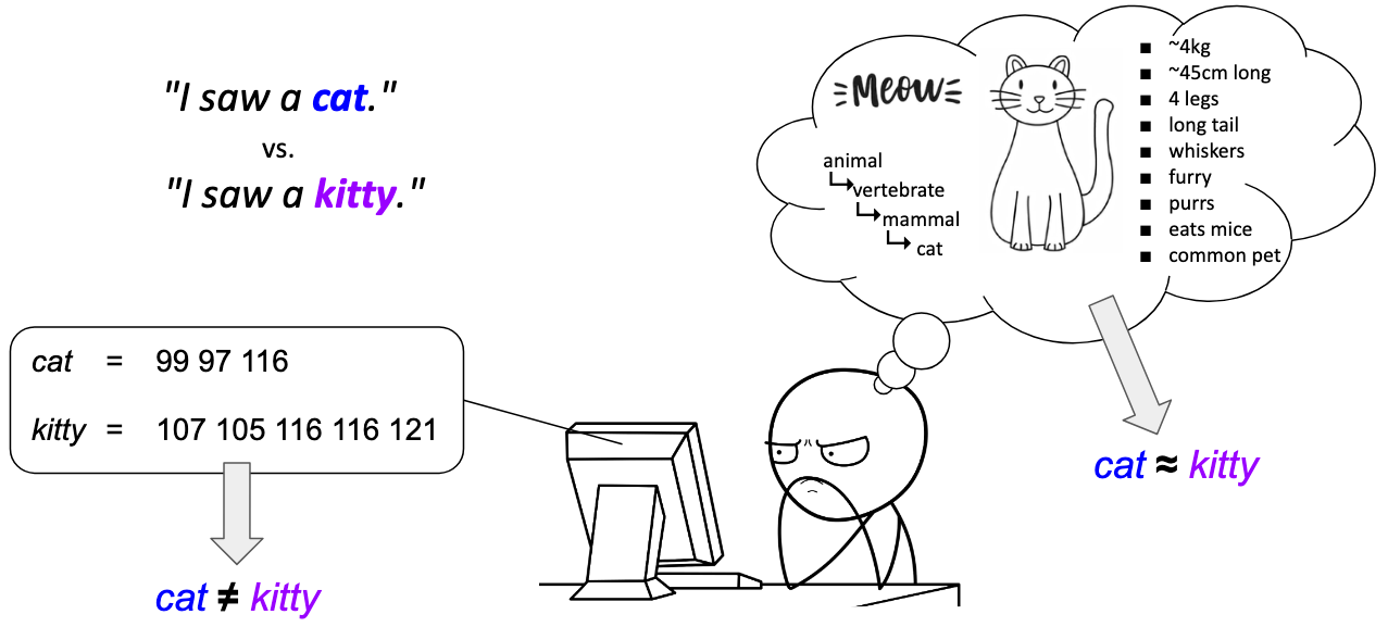
To a machine or algorithm, the two words "cat" and "kitty" are only two strings — in the illustration above, we use the ASCII codes of each letter to show how a machine or algorithm might "see" both words. Most obviously, the two words have a different number of characters. But even if their length would match, the exact characters and corresponding ASCII codes would still differ for different words. Machines have no intrinsic mental representation of words and sentences.
In the most pragmatic sense, to pass words — and therefore also sentence, paragraphs, documents — to a neural network model as valid input, we need to convert words into a fixed-size numerical representation. However, this simple formulation is only a necessary condition but, in practice, often an insufficient condition. To illustrate this problem let's assume we represent each word using vectors containing the ASCII codes of the words in the letter and pad each vector to the longest word (e.g., $10$). With this approach we could represent "cat" and "kitty" as the following embedding vectors:
In principle, each word can now be converted into a fixed-sized numerical representation and indeed be passed to a neural network as a valid input. However, ASCII codes are arbitrary numerical assignments designed for text storage and transmission, not for expressing linguistic relationships. As a result, the numerical distance between character codes or between entire character sequences has no meaningful interpretation: words that are semantically related (e.g., "cat" and "dog") may be far apart in ASCII space, while unrelated words may appear artificially close due to shared characters or similar lengths. For example, the word "hat" would have the vector representation $[104, 97, 116, 0, 0, 0, 0, 0, 0, 0]$ and therefore be much close to "cat" than "kitty".
For neural network-based models, this is a serious limitation because effective learning relies on meaningful notions of similarity and smoothness in the input space. Neural models assume that small changes in input values should correspond to small, interpretable changes in meaning, enabling generalization across related inputs. ASCII-based representations violate this assumption, as they encode surface form rather than conceptual content and fail to reflect semantic or syntactic relatedness between words. Consequently, such representations make it difficult for neural networks to learn patterns about meaning, motivating the use of distributed word representations (embeddings) that place related words close to each other in a learned numerical space.
How Can We Find Good Embeddings?
The core motivation behind word embeddings is to represent words as vectors in a continuous space where each dimension can be interpreted as capturing some latent property or feature that is shared across words. Instead of treating words as isolated symbols, this representation assumes that meaning can be decomposed into multiple underlying factors (e.g., syntactic role, semantic category, or contextual usage) that jointly characterize how words behave in language. By encoding these factors as numerical dimensions, words that share similar properties naturally end up with similar vector representations.
To illustrate this intuition, let's assume we want to find good embedding vectors for animals. In this limited scope, we may come up with the two latent properties or features of an animal being furry and dangerous — of course, the are many more such features (e.g., size, diet, locomotion), but two features is easy to plot — and we express the level of furriness and dangerousness as a values between $0$ and $1$. The table below shows the values for some selected animals; the values are kind of arbitrary and only for illustration purposes.
| furry | dangerous | |
|---|---|---|
| dog | 0.90 | 0.15 |
| cat | 0.85 | 0.10 |
| lion | 0.80 | 0.95 |
| bear | 0.85 | 0.90 |
| cobra | 0.00 | 0.80 |
| cow | 0.75 | 0.10 |
| frog | 0.05 | 0.05 |
| ... | ... | ... |
In other words, can now convert each animal into a $2$-dimensional vector representation, i.e., an embedding:
Since we only have two features, we can easily visualize the embedding vectors in a plot:
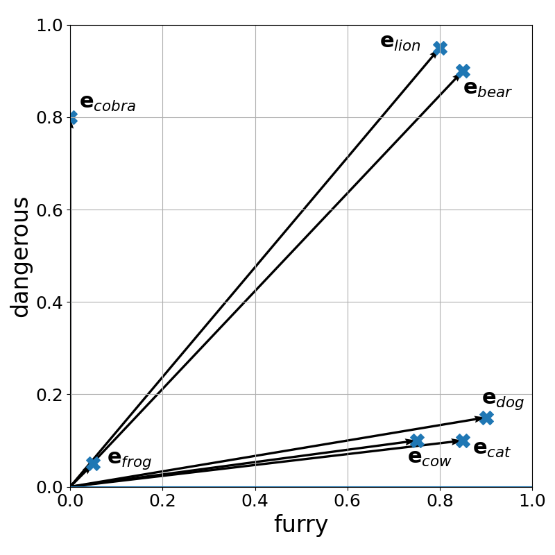
Just by looking at this plot, we can easily see that we can now meaningfully apply suitable vector similarity measures to quantify the similarity or relatedness between words (well, here: animals). Such a vector space makes similarity and relatedness explicit and computationally accessible: words with overlapping properties lie close to each other, while unrelated words are far apart. This structure allows neural models to generalize across vocabulary items, transfer learned patterns from frequent to rare words, and reason about relationships through simple geometric operations. In practice, these properties are not manually defined but are discovered automatically from data, enabling word embeddings to capture rich and nuanced aspects of meaning that are essential for downstream NLP tasks.
Although this is what we want, it is also easy to see which challenges such a manually approach to encode/embed words involve. For example, using furriness and dangerousness to describe arbitrary words such as "movie", "funny", "quickly", "above", and so one does not make meaningful sense. Any many approaches to find good word embeddings would require to answer the following two questions:
- What are meaningful latent properties or features?
- How can we find meaningful values for all properties or features?
Given the plethora and variety of words, a manual approach to find good word embeddings is simply not practical. We therefore need automated, data-driven methods to generate meaningful word embeddings. Although many embedding methods have been proposed, most of them implement the linguistic idea of the Distributional Hypothesis. The Distributional Hypothesis states that words that occur in similar contexts tend to have similar meanings. In other words, if two words frequently appear next to the same neighboring words, they are likely to be semantically related. This hypothesis goes back to works by early linguists and is often captured by their quotes:
"The meaning of a word is its use in the language." (Wittgenstein, 1953)
"If A and B have almost identical environments [...], we say they are synonyms" (Harris, 1954)
"You shall know a word by the company it keeps." (Firth, 1957)
To illustrate idea, consider the following four sentences containing the word "bobotie"; and let's assume you do not know this word:
- "When I was in South Africa, I had bobotie almost every day."
- "We all had bobotie for dinner last night."
- "Although not particularly spicy, bobotie incorporates a variety of flavours"
- "The first recipe for bobotie appeared in a Dutch cookbook in 1609"
Even without knowing the bobotie is a traditional South African dish, just from these sentences alone, it is easy to tell that it is very likely "some" dish, meal, or food. Particularly context words such as "dinner", "spicy", "flavours", "recipe", and "cookbook" are arguably giving string hints. Furthermore, we could, at least in principle, substitute "bobotie" with, say, "stew" and all sentences would still be meaningful — at least semantically when ignoring facts such as the last sentence. This means that "bobotie" and "stew" are considered similar words in the context of the Distributional Hypothesis and should be represented by similar embedding vectors. Word embedding models operationalize this idea by learning vector representations that reflect these context similarities.
Overview & Categorization
The central role of word and text embeddings in modern NLP has driven the development of a wide variety of representation methods, reflecting the many ways in which linguistic information can be encoded and used. At a high level, these methods can be organized by granularity, distinguishing word embeddings, which represent individual tokens in isolation or context, from text embeddings, which aim to capture the meaning of larger units such as sentences, paragraphs, or entire documents. Another key distinction is between sparse and dense embeddings: sparse representations encode text using high-dimensional, interpretable features tied to explicit vocabulary items, whereas dense embeddings compress meaning into low-dimensional, continuous vectors that better capture semantic similarity. Finally, embeddings can be static or contextual. Static embeddings assign a single vector to each word or text regardless of usage, while contextual embeddings adapt representations dynamically based on surrounding context, allowing them to model polysemy and nuanced meaning.
Granularity: Word vs. Text Embeddings
On the most basic level, an embedding vector may represent an individual word or a whole text (e.g., a sentence, a paragraph or a (short) document). Word embeddings capture the meaning of individual words, encoding semantic and syntactic relationships between them. These are useful for tasks where understanding the relationships between words themselves is important, such as word similarity, analogy reasoning, or basic text classification. In contrast, text embeddings aggregate information across multiple words to capture the overall meaning, topic, or sentiment of a text rather than focusing on individual word semantics. This higher-level representation is particularly valuable for tasks like semantic search, document clustering, or summarization, where understanding the broader context and meaning of a piece of text is more important than individual word-level relationships.
Note: Subword-based methods have become extremely common in modern NLP because they address several limitations of word-level embeddings, particularly the handling of rare or out-of-vocabulary words. Instead of representing words as atomic units, subword methods break words into smaller components — such as character n-grams, morphemes, or byte-pair encodings — and learn embeddings for these subunits. This allows models to compose representations for words that were never seen during training by combining the embeddings of their subwords, improving robustness and coverage across diverse vocabularies and languages with rich morphology. With respect to vector representations, subword embeddings are typically combined or aggregated to form a final word or text vector. This approach strikes a balance between granular representation, memory efficiency, and the ability to generalize to unseen or rare words.
Sparsity: Sparse vs Dense Embeddings
Embedding vector word and text embeddings can be broadly distinguished into sparse and dense representations because they embody two fundamentally different ways of encoding linguistic information. On a superficial level, this refers to how the embedding vectors "look" in terms of their size as well as the nature of their values. However, the distinction between dense and sparse vectors have more fundamental effects on their expressiveness when encoding words or text.
Sparse embeddings are high-dimensional (often tens of thousands of dimensions or more) vectors with most elements being $0$. Each dimension usually corresponds to an explicit feature, most commonly to specific word (or token) — in which case the size of the embedding vectors reflects the size of the vocabulary, i.e., the set of unique words/tokens. This sparse structure (high-dimensional + mostly zero values) offer several important advantages, especially in information retrieval and classical NLP settings:
Interpretability and transparency: Each dimension typically corresponds to an explicit, human-understandable feature (e.g., a word or term). This makes it easy to inspect why two texts are considered similar or why a document was retrieved. Sparse embeddings also allow to explicitly control which terms or features are represented (e.g., through stop-word removal or domain-specific vocabularies), which is valuable in specialized or regulated domains.
Exact matching and high precision: Sparse embeddings excel at capturing exact lexical overlap. For example, if a query and document share important terms, sparse representations strongly reflect this, which is crucial for keyword search and precision-oriented tasks. For example, in domains with specific terminologies (e.g., legal, medical, or regulatory texts) it is often crucial that certain words or terms match exactly.
Efficient and stable retrieval: Sparse embeddings integrate naturally with inverted indexes, enabling efficient storage and fast large-scale retrieval, while their deterministic construction ensures stable, reproducible representations without sensitivity to random initialization or training instability.
On the other hand, sparse embedding vectors also come with clear limitations, especially when semantic understanding and robustness are required:
Limited semantic expressiveness and generalization: Sparse embeddings depend on lexical overlap and primarily encode surface-level features, making them ineffective at capturing synonymy, paraphrases, and deeper linguistic structure. For example, sparse embeddings may fail or struggle to capture the semantic similarities between words (e.g., "car" vs. "automobile"), leading to low recall in semantic tasks.
Brittleness to vocabulary variation: Differences in wording, typos, morphological variants, or unseen terms can significantly degrade performance without extensive preprocessing or manual normalization. In practice, this means that strong performance often requires careful, domain-specific preprocessing and weighting schemes, increasing system complexity and maintenance effort.
High dimensionality and poor suitability for semantic tasks: Vocabulary-sized representations are conceptually and computationally unwieldy and perform poorly for similarity-based tasks such as semantic search, clustering, and recommendation.
In practice, dense embedding vectors are more commonly used because they capture semantic relationships between words and texts in a continuous, low-dimensional space. By encoding meaning through distributed representations, dense embeddings can recognize similarity even when there is little or no exact word overlap, allowing models to understand that "car" and "automobile" or "buy" and "purchase" are closely related. This ability to generalize beyond surface-level lexical matching makes dense embeddings especially effective for tasks such as semantic search, clustering, recommendation, and downstream neural NLP models, where robustness to paraphrasing and vocabulary variation is essential.
That said, sparse embeddings remain widely used in settings where high precision, transparency, and controllability are critical. Because each dimension in a sparse representation typically corresponds to an explicit term or feature, it is straightforward to interpret why two documents are considered similar or why a particular result was retrieved. This explainability, combined with strong performance for exact or near-exact matching, makes sparse methods attractive for legal, biomedical, and enterprise search, as well as for compliance-sensitive applications. As a result, rather than being replaced, sparse embeddings often coexist with dense ones, sometimes even combined in hybrid retrieval systems, to balance semantic recall with precision and interpretability.
Context Sensitivity: Static vs. Contextual Embeddings
Static embeddings. A word or text embedding is considered static if the vector representation of the same word or the same text is the same. For example, in case of a word embedding, "bank" will have the same vector representation independently if it is referring to the financial institute or the side of a river in the context of a sentence. Since static embeddings are always the same for the same input (word or text) they can be precomputed and easily shared. This is several advantages:
Efficiency and simplicity: Static embeddings are fast at inference, inexpensive to train, and easy to integrate into downstream models using simple lookup operations.
Low overhead and scalability: They require less memory and computational resources, making them well suited for large-scale or resource-constrained deployments.
Stability and sufficient performance: Their fixed representations are deterministic, easier to debug, and often perform well for tasks where fine-grained contextual meaning is not essential.
However, as the "bank" example already illustrates, static embeddings are limited by their lack of context awareness, as each word or text unit is assigned a single fixed vector that cannot capture multiple meanings or adapt to different usages. This restricts their ability to model fine-grained semantic and syntactic nuances and leads to weaker performance on tasks requiring deep contextual understanding. In addition, static embeddings handle rare or unseen words poorly and are often sensitive to domain shifts, since their representations are tightly coupled to the data on which they were trained.
Contextual embeddings. In contrast to static embeddings, contextual embeddings do generally not assign the same vector representation to a word or text but generate representations dynamically based on the surrounding context, allowing the same word to have different vectors depending on its usage and meaning in a specific sentence or document. In practice, this has several common advantages:
Context-aware representations: Contextual embeddings adapt word or text representations to their surrounding context, effectively handling ambiguity and polysemy (e.g., "bank" will result in different vector representations depending on its use/meaning in a sentence).
Richer linguistic information: They capture fine-grained semantic and syntactic relationships by modeling interactions between words in a sequence.
Improved task performance and robustness: Contextual embeddings generally achieve better results on complex NLP tasks and generalize more well across paraphrases and domains.
On the flip side, contextual embeddings require substantial computational and memory resources because each input must be processed, often through large neural models, which makes both training and inference more expensive and slower compared to static embeddings. This can be a limitation for large-scale or real-time applications, where efficiency is critical. They also introduce engineering challenges such as model versioning, dependency management, and sensitivity to input formulation, where minor changes in wording or punctuation can significantly alter the embeddings. Despite these limitations, their ability to capture nuanced context and improve task performance often outweighs these costs in many modern NLP applications.
Other Characteristics
Apart from granularity (word vs. text), sparsity (sparse vs. dense), and context sensitivity (static vs. contextual), embeddings can be categorized along several other dimensions that reflect how they are trained and used. One common distinction is training objective, which separates embeddings based on whether they are learned through predictive models (e.g., Word2Vec, FastText) that aim to predict surrounding words, or through count-based/statistical methods (e.g., PPMI, LSA) that factorize co-occurrence matrices. Another approach is supervision level, where embeddings may be unsupervised (learned purely from raw text), semi-supervised (leveraging limited labeled data), or task-specific/fine-tuned (adapted to a downstream NLP task). Embeddings can also be categorized by modality or input type. While most embeddings are textual, cross-modal embeddings exist that integrate text with other data types, such as images, audio, or structured knowledge graphs, enabling richer multi-modal representations.
In this notebook, we limit ourselves to textual inputs (word or text) and organize our overview according to the main three dimensions: granularity, sparsity, and context sensitivity. We mention the training objective, supervision level, and other characteristics when discussing the individual embedding methods in more detail.
Word Embeddings
Word embeddings are a central concept in natural language processing because words form the fundamental building blocks of language. Meaning at the level of sentences, paragraphs, or entire documents ultimately emerges from the meanings and interactions of individual words. By assigning each word a numerical representation, word embeddings provide the basic units from which higher-level text representations can be constructed, whether by aggregation, sequence modeling, or more complex neural architectures. High-quality word embeddings therefore have a direct impact on the performance of almost all downstream NLP tasks, as they shape how models perceive and reason about language from the ground up.
In practice, the term "word" is often used as a simplification. Many modern embedding methods do not operate strictly on full words, but on tokens, which may correspond to subwords, character n-grams, or other units derived from tokenization schemes such as Byte Pair Encoding or WordPiece. These subword-based representations help address issues like rare words, morphological variation, and out-of-vocabulary terms. For conceptual clarity, however, it is common to refer to all these units collectively as "words", with the understanding that the underlying models may actually embed smaller or more flexible linguistic units. Thus, in the following, if not stated otherwise, we use the terms "words", "subwords", and "tokens" as synonyms.
Sparse Word Embeddings
One-Hot Encoded Vectors
The most basic way to convert words into a numerical, fixed-sized representation are one-hot encoded vectors. These vectors assign each word in a vocabulary $V$ a unique index. If the vocabulary has $|V|$ distinct words, each word is represented by a $|V|$-dimensional vector that contains all zeros except for a single one at the position corresponding to that word's index.
To give an example, image that our complete text corpus is comprised of only the (shortened) quote by Hamlet "to be or not to be". This gives us a set of unique words, i.e., the vocabulary $V$ = $\{$$be$, $not$, $or$, $to$$\}$. With $|V| = 4$, we know that our one-hot encoded vectors will have a size of $4$. And if we assign each word in $V$ a unique index using the order of words above, we get the following $4$ embeddings:
In practice, when working with large text corpora (often several 10s or even 100s of thousands of unique words) and therefore large vocabularies, the resulting embedding vectors will equally be very large. Still, each embedding vector will only have a single $1$ and the position reflecting the corresponding words; all other entries will be $0$.
While very easy to construct, the main limitations of one-hot encoded word embedding vectors stem from their simplicity. Most importantly, they fail to capture semantic or syntactic relationships between words: all vectors are orthogonal, so semantically related words are no more similar (or dissimilar) than unrelated words. In short, one-hot representations provide no notion of similarity, analogy, or shared meaning. For example consider a large vocabulary $V$ = $\{$$cat$, $kitty$, $table$, $...$$\}$. Thus, the resulting embedding vectors for these three words might look as follows:
Each embedding vector has the same size reflecting the size of the vocabulary $V$; and, of course, we assume that the $1$ is placed at the position in the embedding vector representing the corresponding word. With this representation, no matter which distance or similarity measure you choose, the distance between any two words will always be the same — or even always 0 in case of, e.g., the cosine similarity — whether the two words are semantically related or not.
And secondly, one-hot vectors are high-dimensional and extremely sparse, with dimensionality equal to the vocabulary size. This leads to inefficient memory usage and makes learning statistical patterns harder for models, especially with large vocabularies. Finally, they do not generalize beyond exact word identity: unseen words cannot be represented without extending the vocabulary, and there is no mechanism to share information across words. These drawbacks are a key motivation for dense and distributed word embeddings such as Word2Vec, GloVe, and fastText (as discussed later).
Co-occurrences Vectors
Co-occurrence vectors are an early and intuitive way to represent words based on the Distributional Hypothesis, which states that words appearing in similar contexts tend to have similar meanings. Instead of assigning each word a unique but meaningless identifier (as in one-hot encoding), co-occurrence representations describe a word by how often it appears together with other words in a corpus.
The process involves creating a large co-occurrence matrix (also called a term-term matrix), where each row and column represents a unique word in the vocabulary; this means that the matrix of of size $|V|\times|V|$. We then have to define a context window (e.g., the words immediately surrounding a target word) that to determine "co-occurrence", i.e., the window within two words are said to appear together. The text corpus is then scanned, and a count is incremented in the matrix every time two words appear within the specified context window.
To illustrate the idea, assume that the text snippets below are part of a much larger corpus. Boldface words mark the center words and the underlined words mark their context words. In this example, we assume a context window of size $3$, i.e., the $3$ words preceding and the $3$ word following the center word.
"...has shown that the movie* rating reflects to overall quality...*"
"...the cast of the show* turned in a great performance and..." "...is to get nlp data for ai algorithms on a large scale..." "...only with enough data can ai find reliable patterns to be effective..."*
Based on this corpus we might get a co-occurrence matrix that looks as follows:
| rating | story | data | cast | result | ... | |
|---|---|---|---|---|---|---|
| movie | 2 | 4 | 0 | 1 | 0 | ... |
| show | 6 | 3 | 0 | 2 | 1 | ... |
| nlp | 0 | 1 | 3 | 0 | 4 | ... |
| ai | 1 | 0 | 5 | 0 | 2 | ... |
| ... | ... | ... | ... | ... | ... | ... |
For example, the entry $4$ in the first row and second columns means that the word "story" appeared $4$ times in the context of the word "movie" across the whole corpus. Of course, the complete co-occurrence matrix features a row and a column for each word in the vocabulary; above, we only show a small part of the matrix. Using this organization of the co-occurrence matrix, the embedding vector $\vec{v}_{w}$ for a word $w$ can directly be read from the corresponding row in the matrix; for our four example center words we therefore get:
Just by looking at these vectors, we can already see that the vectors $\mathbf{e}_{\text{movie}}$ and $\mathbf{e}_{\text{show}}$ are more similar to each other than say the vectors $\mathbf{e}_{\text{movie}}$ and $\mathbf{e}_{\text{ai}}$. To quantify this, the table below shows the cosine similarities between all pairs of vectors — but only considering the values shown in the matrix above!
| $\large\mathbf{e}_{\text{movie}}$ | $\large\mathbf{e}_{\text{show}}$ | $\large\mathbf{e}_{\text{nlp}}$ | $\large\vec{v}_{\text{ai}}$ | |
|---|---|---|---|---|
| $\large\mathbf{e}_{\text{movie}}$ | $1$ | $0.80$ | $0.17$ | $0.12$ |
| $\large\mathbf{e}_{\text{show}}$ | $-$ | $1$ | $0.19$ | $0.25$ |
| $\large\mathbf{e}_{\text{nlp}}$ | $-$ | $-$ | $1$ | $0.81$ |
| $\large\mathbf{e}_{\text{ai}}$ | $-$ | $-$ | $-$ | $1$ |
Despite the small example, keep in mind that the vectors are still parsed with a size reflecting the size of the vocabulary $V$ and with most entries being $0$ — after all, for example, there is likely to be a huge number of words the will never appear in the context of word such as "nlp" or "ai".
In general, these co-occurrence vectors based on raw counts are easy to compute and a good attempt to represent words based on the Distributional Hypothesis. However, in practice, raw counts are often skewed by very frequent but also typically less informative words such as determiners (e.g., "a", "an"), conjunctions (e.g., "and", "or", "but"), and prepositions (e.g., "from", "to", "by"). This issue can be addressed in various ways. A straightforward approach is to remove such less informative words from the vocabulary, and therefore the co-occurrence matrix and the context window. Alternative approaches include reweighting and/or normalization schemes to limit the influence of less informative words on the entries in the co-occurrence matrix. But these extensions to the basic concept of co-occurrences vectors are beyond this overview here.
Dense Word Embeddings
Static Dense Word Embeddings
Converting Sparse to Dense Vectors
One general and common way to create static dense embedding vectors is to convert static sparse embedding vectors by apply linear dimensionality reduction to a co-occurrence matrix. The most widely used strategy is Singular Value Decomposition (SVD), where the matrix is factorized and only the top-$k$ singular components are retained. This produces low-dimensional dense vectors that capture the dominant co-occurrence patterns in the data, as in Latent Semantic Analysis (LSA). Closely related approaches include truncated SVD and Principal Component Analysis (PCA), which similarly project high-dimensional sparse vectors into a compact continuous space while preserving as much variance or structure as possible. Beyond linear methods, non-linear dimensionality reduction techniques such as autoencoders or neural factorization models can also be used to learn dense representations, although classical linear methods remain popular due to their simplicity, interpretability, and strong connection to distributional semantics.
These dimensionality reduction methods for obtaining dense embeddings have several structural limitations compared to predictive embedding models like Word2Vec, GloVe, or fastText (discussed below). Most importantly, they rely on global matrix construction and factorization, which is memory-intensive and computationally expensive for large vocabularies and corpora. This makes them difficult to scale and update incrementally when new data arrives. In addition, these methods typically depend on fixed co-occurrence statistics and linear projections, which limits their ability to model more complex, non-linear semantic relationships present in language. Furthermore, embeddings derived via dimensionality reduction are usually static and word-level only, assigning a single vector per word and offering no built-in mechanism for handling rare or unseen words. As a result, while dimensionality reduction techniques are conceptually elegant and historically important, they are generally less flexible and less expressive than modern embedding approaches.
Word2Vec
Word2Vec, introduced by Mikolov et al. (2013), is a family of neural embedding models that learn dense, low-dimensional vector representations of words from large text corpora by exploiting their surrounding contexts. By capturing distributional patterns of word co-occurrence, Word2Vec embeddings encode semantic and syntactic relationships, enabling words with similar meanings to be close to each other in vector space.
In its core, Word2Vec is implemented as a word classification task where the goal is to train a model that can predict word relationships based on their contexts. The figure below illustrates the general architecture assuming a single word as input and a single word as output. The Word2Vec model can be implemented as a shallow neural network contain one hidden layer — represented by input weight matrix $\mathbf{U}$ — and one output layer — represented by input weight matrix $\mathbf{V}$ — This classification setup is essential because it enables Word2Vec to learn semantic word embeddings indirectly through prediction. By training to correctly classify words in context, the model adjusts its internal word vectors, captured by $\mathbf{U}$ and $\mathbf{V}$ so that words appearing in similar contexts have similar representations. Thus, while Word2Vec’s ultimate goal is not classification per se, framing it as such provides a simple and effective learning objective for capturing the statistical structure of language.
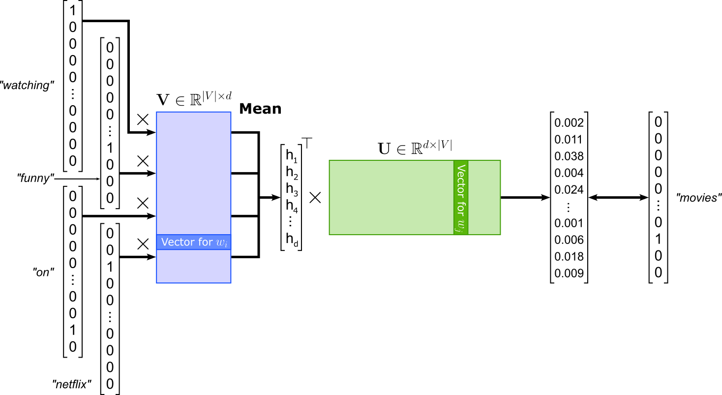
While there are different model implementations of Word2Vec typically focusing on improving efficiency, the two fundamental architectures of Word2Vec are Continuous Bag-of-Words (CBOW) and Skip-gram. The CBOW model takes as input a set of context words (typically words within a fixed window around the target) and aims to predict the center word. The "bag-of-words" term refers to the fact that the order of context words is ignored; only their presence matters. For example, in the sentence "we were watching funny movies on netflix last weekend", if the window size is 2 and the target word is "movies", the context words would be "watching", "funny", "on", and "netflix" (again, CBOW ignores the actual order). For this example, the training sample might look as follows — keep in mind that the order of the context words does not matter, even when shown as a list here:
(["watching", "funny", "on", "netflix"], "movies")
In terms of architecture, CBOW uses a shallow neural network with one hidden layer. Each input context word is represented as a one-hot vector, which is mapped to its embedding vector via the input weight matrix. These embedding vectors are then averaged (or summed) to form a single context representation, which is passed through the output layer to predict the probability distribution over all words in the vocabulary. The model is trained to maximize the probability of the correct target word given the context words. The figure below illustrates the overall CBOW architecture.
The Skip-gram model of Word2Vec is the "opposite" of the CBOW model: Instead of predicting the center or target word given the context words like in CBOW, Skip-gram is modeled to predict the context words given the center words. Using the same example, given the word "movies", Skip-gram learns to predict the context words "watching", "funny", "on", and "netflix". Again, the order of the context words does not matter. The model architecture of SKip-gram is very similar to CBOW; see the figure below. Since Skip-gram takes in a single word, there is no longer a need to compute the average of multiple inputs embeddings. In contrast, Skip-gram has to compute multiple losses with respect to each predicted context word.
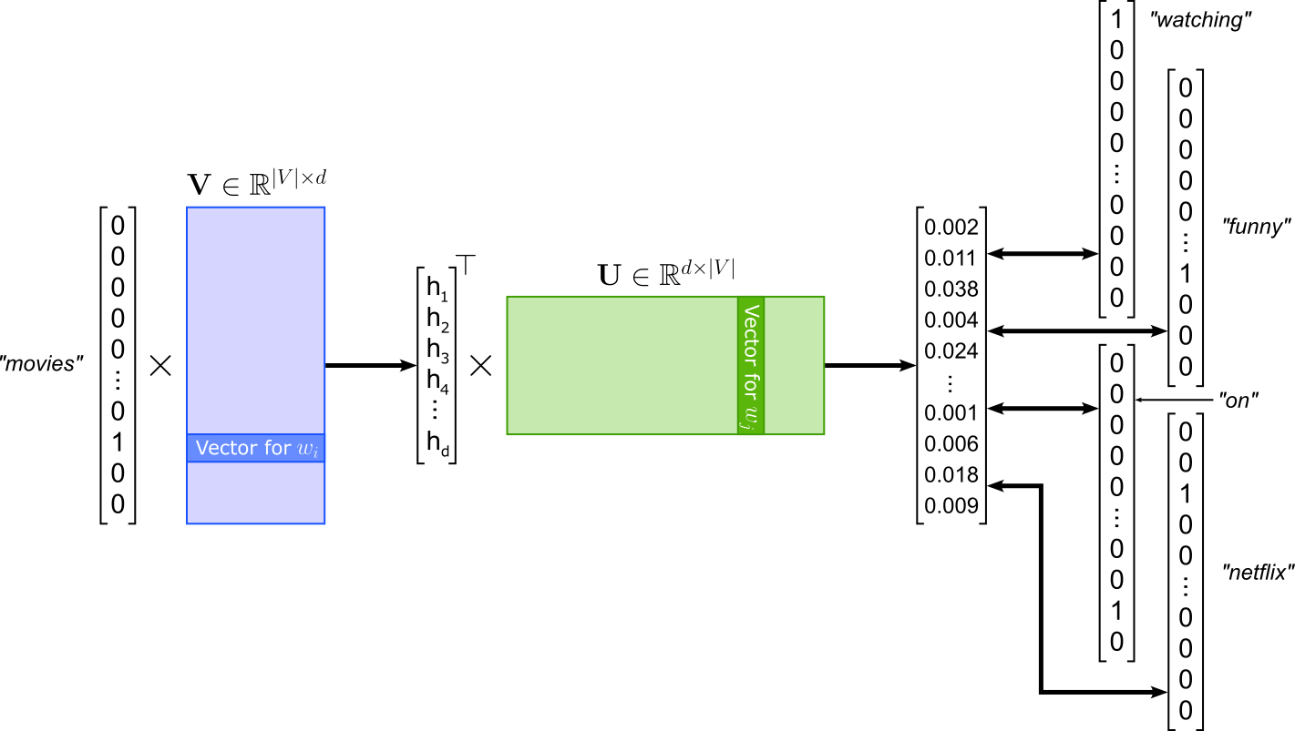
Since the losses between a center word and all context words are independent from each other, we can treat each (center, context) pair as its own training samples. This means, given the example illustrated in the figure above with a window size of $2$, we get the following $4$ training samples:
("movies", "watching")
("movies", "funny")
("movies", "on")
("movies", "netflix")
Both CBOW and Skip-gram have the same underlying training objective. If $\mathbf{v}_i \in \mathbf{V}$ denotes the input embedding vector for a word $w_i$, and $\mathbf{u}_j \in \mathbf{U}$ the output embedding vector of a word $w_j$, both models try to minimize the dot product $\mathbf{u}_{j}^\top \mathbf{v}_i$. Intuitively, this means that the embedding vectors of center words and context words become more and more similar during the training of both models. Notice that this is not really what we are looking for. For example, we are not directly interested in the case where the embedding vectors for the words "movie" and "funny" are similar. However, this explicit training objective implies that (center) words that often appear in very similar contexts will also have similar embedding vectors. To see, this consider the phrase "watching funny videos on YouTube", with "videos" being the center words. Since (a) the words "movies" and "videos" often appear in (very) similar contexts, and (b) both their embedding vectors will be similar to embedding vectors of those shared context words, the embedding vectors for "movies" and "videos" will also be similar.
Notice that in both CBOW and Skip-gram, each word is associated with two distinct vector representations: an input embedding in $\mathbf{V}$ and an output (target) embedding in $\mathbf{U}$. As a result, the models learn two embedding matrices, reflecting the asymmetric roles words play when they appear as predictors versus prediction targets. After training, several strategies exist to obtain a single embedding per word. The most common approach is to discard the output embeddings and keep only the input embeddings, which empirically work well for many downstream tasks. Alternatively, one can use only the output embeddings, or combine both vectors, for example by averaging or concatenating them, to capture information from both roles. In practice, the choice depends on the task, but using the input embeddings alone has become the de facto standard due to its simplicity and strong performance.
GloVe
GloVe (Global Vectors), introduced by Pennington et al. (2014), is a word embedding method that learns dense vector representations by modeling global word-word co-occurrence statistics from a corpus.
| ... | france | germany | city | rain | ... | $\sum$ | |
|---|---|---|---|---|---|---|---|
| ... | ... | ... | ... | ... | ... | ... | ... |
| paris | ... | 250 | 30 | 460 | 10 | ... | 1600 |
| berlin | ... | 20 | 300 | 480 | 13 | ... | 1900 |
| ... | ... | ... | ... | ... | ... | ... | ... |
However, instead of working with these raw co-occurrence counts, GloVe uses co-occurrence probabilities because probabilities normalize for word frequency and make statistics comparable across different target words — similar why sparse embeddings based on co-occurences reweigh or scale the raw counts (see above). Raw counts are dominated by very frequent words, whereas probabilities reflect how informative a context word is for a given target word, independent of how often the target occurs overall.
The co-occurrence probabilities are the conditional probabilities $P_{ij} = P(j|i) $ of seeing a context word given $w_j$ a center (or target) word $w_i$. For example, the co-occurrence probability $P_{paris,france}$ or $P(france|paris)$ is the conditional probability that the word "france" is in the context of "paris". $P_{ij}$ is computed as the relative frequency of seeing $w_j$ in the context of $w_i$:
where $X_{ij}$ is the number of times word $w_j$ appears in the context of word $w_i$, and $X_{i}$ is the total number of words appearing in the context of $w_i$. To show some example, let's compute the two co-occurrence probabilities $P_{paris|france}$ and $P_{paris|germany}$ based on the counts $X_{ij}$ and $X_{i}$ given by the co-occurrence matrix containing the raw counts given above.
Given that Paris is the capital of France, it seems intuitive that the co-occurrence probability $P_{paris,france}$ is much higher than $P_{paris,germany}$. Computing these probabilities for all pairs of center and context words, we get the following matrix containing all co-occurrence probabilities — of course, the matrix below only shows the probabilities which can be computed with the available raw counts in our example.
| ... | france | germany | city | rain | ... | |
|---|---|---|---|---|---|---|
| ... | ... | ... | ... | ... | ... | ... |
| paris | ... | 0.156 | 0.019 | 0.287 | 0.006 | ... |
| berlin | ... | 0.011 | 0.158 | 0.253 | 0.007 | ... |
| ... | ... | ... | ... | ... | ... | ... |
However, like that raw counts, the co-occurrence probabilities are heavily influenced by how frequent a context word $w_j$ is overall. For example, we would expect that the word "the" is a frequent context word of many to most other words, including "paris". As a consequence, the probability $P_{paris,the}$ will also be high just like $P_{paris,france}$. However, "france" arguably carries much more semantic information about "paris" then "the". To address this, GloVe considers the ratio $P_{ik}/P_{jk}$ to capture how strongly a context word $w_k$ is associated with word $w_i$ compared to word $w_j$. Using this ratio of probabilities has several advantages. Firstly, the absolute count of the context word $w_k$ does no longer matter as it cancels out:
And secondly, focusing on ratios of co-occurrence probabilities rather than raw probabilities highlight relative differences between words in a given context, which are more informative for capturing meaning. By modeling ratios, GloVe ensures embeddings reflect the semantic contrasts between words, which is essential for encoding meaningful linear relationships in vector space. For our example, computing the ratios $P_{paris,k}/P_{berlin,k}$ for our four context words, we get:
| k=france | k=germany | k=city | k=rain | |
|---|---|---|---|---|
| $\Large\frac{P_{paris,k}}{P_{berlin,k}}$ | 14.844 | 0.119 | 1.138 | 0.913 |
The are two main cases for the ratio values:
$P_{ik}/P_{jk} \gg 1$ or $P_{ik}/P_{jk} \ll 1$: In both these cases, the two probabilities $P_{ik}$ and $P_{jk}$ are very different, indicating that the context $w_k$ is very useful for distinguishing between the words $w_i$ and $w_j$.
$P_{ik}/P_{jk} \approx 1$: Here, the two probabilities $P_{ik}$ and $P_{jk}$ are quite similar, indicating that the context $w_k$ is not useful for distinguishing between the words $w_i$ and $w_j$. Note that this happens if both probabilities are large (the context word is relevant to both $w_i$ and $w_j$) or both probabilities are low (the context word is irrelevant to both $w_i$ and $w_j$). However, since we want to highlight relative differences, both cases capture the same information.
In short, these observations show that the ratios $P_{ik}/P_{jk}$ are useful for learning meaningful word embeddings. GloVe now aims to learn vectors for each word — in their roles as center and context words — such that their dot product relates directly to their probability of co-occurrence; more specifically, their log probabilities. Again, if $\mathbf{u}_j$ denotes the context embedding of word $w_j$ and $\mathbf{v}_i$ denotes the input embedding of the center word $w_i$, the learning objective of GloVe is to find $\mathbf{u}_j$ and $\mathbf{v}_j$ such that:
Through mathematical derivation involving properties of vector differences and homomorphisms, the this training objective can be rewritten relate the dot product of word vectors to the logarithm of their co-occurrence counts $X_{ij}$ (instead of their co-occurrence probabilities $P_{ij}$). The loss function implementing training objective also includes additional considerations to down-weights very frequent co-occurrences (like "the" appearing with "a"), preventing them from dominating the training objective, as well as extremely rare co-occurrences, which might be noisy or unreliable. However, these mathematical details go beyond our discussion here.
Like Word2Vec, GloVe learns two word embedding vectors for each word $w_i$ depending on its role: as center (or target) word ($\mathbf{v}_i$) and as context word ($\mathbf{u}_i$). However, unlike in Word2Vec (where typically only $\mathbf{v}_i$ is used), in GloVe the most common approach is the compute the sum of both embeddings to get the final vector representation $\mathbf{e}_i$ of word $w_i$, i.e., $\mathbf{e}_i = \mathbf{v}_i + \mathbf{u}_i$. While alternatives — using only $\mathbf{v}_i$ (i.e., $\mathbf{e}_i = \mathbf{v}_i$), only $\mathbf{u}_i$ (i.e., $\mathbf{e}_i = \mathbf{u}_i$), the average (i.e., $\mathbf{e}_i = \frac{1}{2}(\mathbf{v}_i + \mathbf{u}_i)$), or the concatenation (i.e., $\mathbf{e}_i = \left[\mathbf{v}_i; \mathbf{u}_i\right]$) — are possible, the simple sum emperically shows the best result when the GloVe embeddings are used for downstream tasks.
fastText
fastText, developed by Facebook,s AI Research (FAIR) lab, serves as an extension of the Word2Vec framework, specifically building upon the CBOW and Skip-gram architectures. While traditional Word2Vec models treat each word as an atomic, indivisible entity, fastText introduces a more granular approach by representing each word as a bag of character n-grams. By incorporating these sub-word features, fastText allows the model to capture the internal structure and morphology of words. This architectural shift provides two significant advantages over its predecessors: it can generate high-quality embeddings for rare words that appear infrequently in the training data, and it effectively solves the Out-of-Vocabulary (OOV) problem. Even if a word was never seen during training, fastText can still construct a vector for it by summing the representations of its constituent n-grams, making it exceptionally robust for morphologically rich languages and datasets with frequent misspellings.
In the standard fastText implementation, only the input words (the words used as context in Skip-gram or the window words in CBOW) are split into n-grams. The output words (the target words being predicted) are typically treated as distinct, whole entities. The size of the n-grams is a hyperparameter. For example, with $n=3$ (i.e., $3$-grams), the word "netflix" would be decomposed into sub-word sequences like "<ne", "net", "etf", "tfl", "fli", "lix", and "ix>". The angled brackets are important to indicate word boundaries, helping the model distinguish between subwords that appear at different positions. For example, the word "get" cannot be split into $3$-grams, but the model needs to able to distinguish the whole word from "get" being a $3$-gram in, say, "forgettable". Apart from the n-grams, fastText still takes in each input word as a whole word as well. Thus, using $3$-gram, our CBOW training sample from above will look as follows for fastText:
(["<wa", "wat", "atc", "tch", "chi", "hin", "ing", "ng>", "<watching>", "<fu", "fun", "unn", "nny", "ny>", "<funny>", "<on", "on>", "<on>", "<ne", "net", "etf", "tfl", "fli", "lix", "ix>", "<netflix>"], "movies")
Similarly, the Skip-gram inputs that include all $3$-grams for fastText, would change to:
(["<mo", "mov", "ovi", "vie", "ies", "es>", "<movies>"], "watching")
(["<mo", "mov", "ovi", "vie", "ies", "es>", "<movies>"], "funny")
(["<mo", "mov", "ovi", "vie", "ies", "es>", "<movies>"], "on")
(["<mo", "mov", "ovi", "vie", "ies", "es>", "<movies>"], "netflix")
Again, the general architectures of CBOW and Skip-gram remain the same. The only difference is now that the vector representation of each input word is now the sum of the words embedding vectors as well as of all its n-grams' embedding vectors. More formally, recall that in basic CBOW and Skip-gram, the training objective is to minimize the dot product $\mathbf{u}_{j}^\top \mathbf{v}_i$, where $\mathbf{v}_i \in \mathbf{V}$ is the input embedding vector for a word $w_i$, and $\mathbf{u}_j \in \mathbf{U}$ the output embedding vector of a word $w_j$. Now, in fastText, let $\mathcal{G}_i$ denote all n-grams $g\in\mathcal{G}_i$ of the word $w_i$, and let $\mathbf{z}_g \in \mathbf{Z}$ be the vector representation of n-gram $g$; $\mathbf{Z}\in \mathbb{R}^{|H|\times d}$ is the new weight matrix containg the vector representations for all n-grams $H$. With that, the new dot product to be minimized during training is now:
One of the design goals of fastText is the handle unseen words, i.e., to generate meaningful vector representation during inference time for word that were not part of the training corpus. For example, let's assume we want to embed the word "youtube" which did not appear in the training data. Of course, "youtube" will not have a corresponding entry in the input embedding matrix $\mathbf{V}$ for the whole word. However, the assumption is that a majority of the, say, $3$-grams "<yo", "you", "out", "utu", "tub", "ube", and "be>" will be known, i.e., be in $\mathbf{Z}$.
Of course, unseen words might also result in unseen n-grams. However, fastText does not ignore new n-grams at inference time as this would throw away exactly the information fastText was designed to capture, i.e., subword structure. Instead, fastText uses hashing guarantees that every possible n-gram always maps to some embedding vector, even if that n-gram was never seen during training. More concretely, fastText does not maintain an explicit lookup table of known n-grams. Instead, it stores a fixed-size array of embedding vectors (hash buckets) that were trained using all n-grams encountered during training. When a new n-gram appears at inference time, the same hash function is applied, and the resulting index points to one of these already-trained buckets. That bucket's vector has been updated during training by other n-grams that happened to hash to it. Due to this parameter sharing, the new n-gram inherits a representation that reflects similar character patterns learned from the training data.
Ignoring unseen n-grams would lead to systematically weaker representations for unseen words, especially those composed of novel but informative character sequences. Hashing instead provides a smooth generalization mechanism: unseen n-grams are not treated as "unknown" but are mapped into the same embedding space as known ones, with collisions acting as a form of regularization. As long as the number of hash buckets is sufficiently large, collisions are sparse enough that this approximation works well in practice, allowing fastText to remain efficient while still producing meaningful embeddings for previously unseen words.
Contextual Dense Word Embeddings
ELMo (Embeddings from Language Models)
ELMo (Embeddings from Language Models) is a deep contextualized word embedding approach that represents words as functions of the entire input sentence rather than as fixed vectors. Unlike traditional static embeddings such as Word2Vec or GloVe, which assign a single representation to each word regardless of context, ELMo captures how a word's meaning changes depending on its surrounding words. It does so by training a deep bidirectional language model (biLM) that reads text both left-to-right and right-to-left, allowing it to model rich syntactic and semantic information at multiple levels.
ELMo trains a RNN-based language model based on the next-word prediction task using a self-supervived setup: the target sequence of a training sample is the same as the input sequence only shifted to the left by $1$ token. As the concrete RNN architecture, the original ELMo model uses a bidirectional LSTM (Long Short-Term Memory) network with $2$ layers. The figure below illustrates the overall setup:
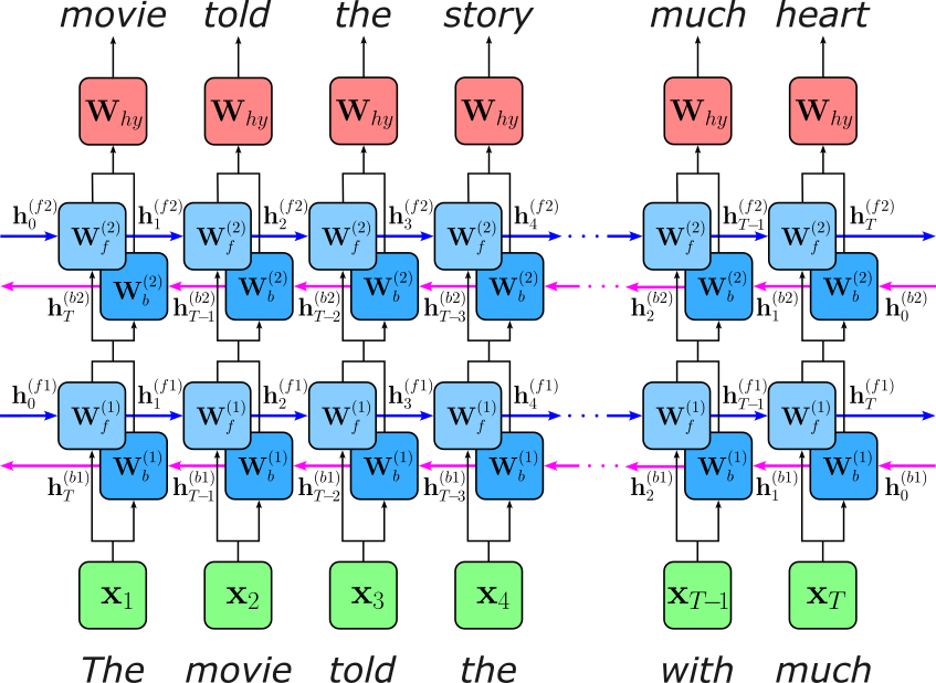
Using a bidirectional LSTM allows ELMo to construct word representations that depend on both left and right context, which is crucial for capturing how meaning varies with usage. Many words are ambiguous when viewed from only one direction (e.g., "bank", "charge"), and relying solely on past context can be insufficient to disambiguate them. By combining a forward LSTM that summarizes preceding words with a backward LSTM that summarizes following words, ELMo produces embeddings that encode richer syntactic and semantic information, such as long-range dependencies, agreement, and phrase-level structure. This bidirectional context is especially beneficial for downstream tasks like named entity recognition or question answering, where cues often appear after the word being interpreted.
This design is suitable for ELMo precisely because the model is not intended to generate text, but to serve as a feature extractor for contextual word embeddings. Unlike generative language models, which must respect causality and predict tokens sequentially, ELMo is applied to complete sentences that are fully observed. This allows it to "peek" at future words without violating any constraints. As a result, the bidirectional LSTM can leverage the entire sentence to compute embeddings, yielding more informative representations than unidirectional models while remaining perfectly aligned with ELMo’s goal of understanding text rather than producing it.
After training, ELMo embedding $\mathbf{e}_t$ for the $t$-th word in an input sequence is not taken from a single layer or a single vector table, but are constructed dynamically as "some" combination of the internal hidden states of model, sometimes including the uncontextualized embedding $\mathbf{h}_t^{(0)}$ (i.e., the initial embedding that serves as input for the first LSTM layer). The figure below shows the overall approach, where $\mathbf{h}_t^{(1)}$ is the output of the first LSTM layer as the concatenation of the hidden states of the forward and backward direction; similarly, $\mathbf{h}_t^{(2)}$ is the output of the second LSTM layer.
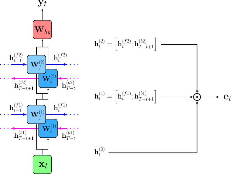
The most basic approach is to use the output of the last LSTM layer as the final embedding, i.e., $\mathbf{e}_t = \mathbf{h}_t^{(2)}$. The more generalized approach computes the final embedding $\mathbf{e}_t$ as the weighted sum of the three possible outputs:
The weights $s_i$ are learned but not during ELMo's language-model pretraining. They are learned during training for each downstream task. During downstream training, gradients from the task loss (e.g., NER, QA, classification) update these scalars so the model learns which layers are most useful for that task. For example, syntactic tasks often place more weight on lower layers, while semantic tasks emphasize higher layers. Importantly, the ELMo language model parameters are usually frozen, so only the layer-mixing weights and the downstream model parameters are trained. This makes ELMo efficient and stable, while still allowing flexibility: each task learns its own optimal mixture of representations without retraining the entire language model.
The scaling factor $\gamma$ learned, task-specific scalar that controls the overall magnitude of the ELMo embedding after the layer representations have been combined. The purpose of $\gamma$ is to let the downstream model rescale the ELMo representation so it fits well with other input features or embedding sources (e.g., static word embeddings or character features) used in the task. Without this scaling, the combined ELMo vector might have a magnitude that is too large or too small relative to other inputs, which can make optimization harder. Like the weights $s_i$, the scaling factor $\gamma$ is learned during downstream task training, not during ELMo pretraining. Conceptually, it acts as a learned "gain" parameter, giving the model flexibility to decide how strongly ELMo embeddings should influence the task — ranging from subtle auxiliary features to dominant representations — while keeping the pretrained language model itself fixed.
BERT (Bidirectional Encoder Representations from Transformers)
BERT is a widely used contextual embedding model that represents words as vectors conditioned on their full surrounding context. Unlike earlier static embeddings such as Word2Vec or GloVe, but similar to ELMo, BERT produces different embeddings for the same word depending on how it is used in a sentence, allowing it to capture polysemy and subtle semantic distinctions. This context sensitivity is achieved by pretraining the model on large corpora using objectives such as masked language modeling, which encourages the model to infer missing tokens from both left and right context simultaneously.
Architecturally, BERT is based on an encoder-only Transformer, consisting of stacked self-attention and feed-forward layers without a decoding component. The self-attention mechanism enables each token to directly attend to all other tokens in the input sequence, making BERT inherently bidirectional and well suited for understanding tasks rather than text generation. As a result, BERT embeddings encode rich syntactic and semantic information and can be used effectively for a wide range of downstream NLP tasks, either as fixed contextual representations or fine-tuned end-to-end for task-specific objectives. BERT is trained using two learning objectives:
Masked Language Model (MLM): During training, a fixed proportion of input tokens (typically around 15%) is selected at random and their original identities are hidden from the model. These selected tokens are replaced with a special
[MASK]token most of the time, and the model is then trained to predict the original tokens using the surrounding context on both the left and right. The learning objective is to maximize the likelihood of the correct original tokens at the masked positions, effectively turning the task into a multi-class classification problem over the vocabulary. This objective forces BERT to build representations that integrate information from the entire sentence, since the masked token cannot be predicted using only local or unidirectional context.Next Sentence Prediction (NSP): A training sample for BERT contains pairs of sentences. In 50% of the cases, the second sentence truly follows the first one in the original corpus; in the other 50%, it is a randomly sampled sentence from the corpus. The two sentences are concatenated into a single input sequence, separated by a special
[SEP]token, and a classification token[CLS]is added at the beginning. The model is then trained to predict whether the second sentence is the actual continuation of the first. The goal of NSP is to encourage BERT to capture inter-sentential coherence and discourse-level information, which is important for tasks involving sentence pairs, such as question answering and natural language inference. By framing this as a binary classification problem over the[CLS]representation, BERT learns to encode not only the meaning of individual sentences but also how sentences relate to each other in context.
The figure below illustrates the overall training setup of BERT with both learning objectives.
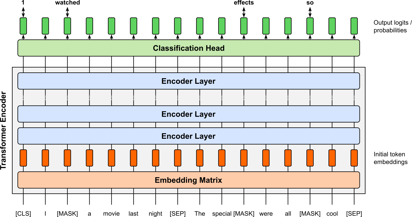
During training, the total loss is determined by the two learning objectives: The MLM loss is computed only over the masked token positions. For each masked position, BERT predicts a probability distribution over the vocabulary, and the loss is the sum (or average) of the cross-entropy between these predictions and the true original tokens. Unmasked tokens do not directly contribute to the MLM loss, although they influence it indirectly through self-attention by providing context. The NSP loss is a binary classification loss computed from the final hidden state of the [CLS] token. The model predicts whether the second segment is the actual next sentence or a random one, and a cross-entropy loss is applied to this prediction. The overall pretraining loss is the sum of the MLM loss and the NSP loss, jointly optimizing BERT to learn both token-level contextual representations and sentence-level relationships.
After training, for a given input sequence, the BERT model outputs a sequence of hidden states (one vector per input token) from each Transformer encoder layer. Each of these vectors encodes the meaning of its corresponding token conditioned on the entire input sequence via self-attention. In practice, the token-level embedding for each input token is typically taken from the final encoder layer, though some applications combine representations from multiple layers (e.g., by concatenation or averaging) to capture different levels of linguistic information.
In addition to token-level embeddings, BERT also produces a special sequence-level embedding associated with the [CLS] token. This vector is commonly used as a holistic representation of the entire input sequence or sentence pair, especially for classification tasks. Importantly, because BERT uses subword tokenization (e.g., WordPiece), a single word may correspond to multiple token embeddings; word-level representations are often obtained by pooling over these subword vectors.
Since the original BERT model was introduced, many BERT variants have been proposed to improve performance, efficiency, or scalability by modifying the training objectives, architecture, or training data. RoBERTa (Robustly Optimized BERT Pretraining Approach) shows that BERT can be significantly improved by training longer on much larger corpora, removing the Next Sentence Prediction (NSP) objective, and using larger batch sizes and dynamic masking. DistilBERT focuses on efficiency: it uses knowledge distillation to train a smaller, faster model that retains most of BERT’s performance while reducing inference cost. ALBERT (A Lite BERT) targets parameter efficiency by factorizing embedding matrices and sharing parameters across layers, allowing much deeper models with far fewer parameters.
Other variants continue this trend of specialization. For example, ELECTRA replaces MLM with a discriminator-based objective that learns to detect replaced tokens, achieving strong performance with less computation, while DeBERTa improves attention modeling by disentangling content and positional information. Together, these variants demonstrate that BERT's core encoder-only Transformer architecture is flexible and can be adapted to different trade-offs between accuracy, speed, and memory usage. The following table provides a quick overview to popular BERT variances at a glance.
| Model | Approx. Parameters | Training Corpus Size | Key Differences from BERT | Main Advantage |
|---|---|---|---|---|
| BERT-base | ~110M | ~16 GB (BooksCorpus + Wikipedia) | MLM + NSP, standard encoder-only Transformer | Strong general-purpose baseline |
| RoBERTa-base | ~125M | ~160 GB | No NSP, dynamic masking, longer training | Higher accuracy than BERT |
| DistilBERT | ~66M | Same as BERT (via distillation) | Fewer layers, knowledge distillation | Faster and lighter |
| ALBERT-base | ~12M | ~16 GB | Parameter sharing, factorized embeddings | Memory efficient |
| ELECTRA-small | ~14M | ~16 GB | Replaced-token detection instead of MLM | Compute efficient training |
| DeBERTa-base | ~140M | ~160 GB | Disentangled attention, improved position encoding | Strong performance on reasoning tasks |
This landscape highlights how BERT-style embeddings have evolved into a family of models optimized for different practical constraints and application needs.
Beyond BERT — Beyond Encoder-Only
BERT was a landmark model in NLP as it was the first widely successful approach to learn contextual word embeddings using the Transformer architecture. However, the subsequent explosion of decoder-only LLMs and encoder-decoder LLMs has broadened the landscape for learning word (and text) embeddings. These models, initially optimized for text generation, can be adapted to produce contextual embeddings using techniques like pooling hidden states or contrastive fine-tuning. As a result, a wide range of alternative methods — spanning encoder-only, decoder-only, and encoder-decoder architectures — have emerged to generate embeddings tailored to semantic search, clustering, or task-specific representation learning.
Encoder-decoder architectures: Learning word embeddings from encoder-decoder architectures (e.g., T5, BART) is relatively straightforward since we still have the encoder. Much like in BERT, the encoder hidden states are typically used, much like in BERT. Since the decoder is primarily optimized for autoregressive generation conditioned on the encoder output, its hidden states are less commonly used for standalone word embeddings, although they can be useful when embeddings are needed in the context of sequence-to-sequence tasks. Additionally, some approaches fine-tune encoder-decoder models with contrastive or supervised objectives to produce embeddings optimized for semantic similarity or retrieval tasks.
Decoder-only architectures: Learning word embeddings from decoder-only architectures (such as GPT-style models) is less straightforward than with encoder-only models because these architectures are designed for autoregressive, left-to-right text generation. By default, each token's hidden state only attends to preceding tokens, producing unidirectional contextual embeddings. For many downstream tasks requiring bidirectional context, this can be limiting. To better adapt decoder-only architectures for embedding tasks, several strategies are employed. One approach is removing or modifying causal masking, allowing each token to attend to all positions in the input, effectively mimicking bidirectional attention as in encoder-only models. Another approach is introducing masked language modeling (MLM) or contrastive objectives during fine-tuning, which encourages the model to learn embeddings that capture semantic similarity rather than solely predicting the next token.
This evolution demonstrates that while BERT was the pioneering Transformer-based embedding model, the field has rapidly diversified, leveraging the flexibility of modern LLM architectures to produce high-quality, context-aware embeddings in many different ways. A wide range of LLM-based word (and text) embedding models have been proposed, with a more detailed overview beyond our scope in this notebook. However, for further reading, here are some references to popular approaches
- Generative Representational Instruction Tuning (Muennighoff et al., 2024)
- NV-Embed: Improved Techniques for Training LLMs as Generalist Embedding Models (Lee et al., 2024)
- LLM2Vec: Large Language Models Are Secretly Powerful Text Encoders (BehnamGhader et al. 2024)
- Causal2Vec: Improving Decoder-only LLMs as Versatile Embedding Models) (Lin et al., 2025)
- Qwen3 Embedding: Advancing Text Embedding and Reranking Through Foundation Models (Zhang et al., 2025)
Note: While many word embedding models are accompanied by detailed scientific publications, there is also a growing trend of popular models being released by companies and organizations without full technical disclosure. In such cases, the models may be shared via APIs, pretrained weights, or online repositories, but the exact details of the training data, architecture modifications, hyperparameters, or pretraining objectives are not fully documented. Examples include some commercial embeddings released by OpenAI, Cohere, or proprietary search and recommendation embeddings, where the primary goal is practical usability rather than academic reproducibility.
Text Embeddings
Text embeddings extend the idea of word embeddings by representing larger units of language such as sentences, paragraphs, or entire documents, as single vector representations. While word embeddings capture the meaning of individual tokens, they cannot directly encode how words interact or combine to form the meaning of longer texts. Text embeddings address this limitation by aggregating, transforming, or contextualizing the information from multiple words into a fixed-length vector that reflects the semantics of the full text. This enables downstream tasks, such as semantic search, clustering, or classification, to operate on entire texts rather than relying solely on word-level comparisons, providing a more holistic and meaningful representation of language.
Most text embedding models designed for sentences, paragraphs, or entire documents apply a fixed mapping from text to vector once training is complete. At inference time, the model parameters are frozen and the embedding is computed solely from the input text, without conditioning on surrounding documents, user intent, or task-specific signals. As a consequence, the same sentence or paragraph will always be mapped to the same vector representation, provided the model and preprocessing remain unchanged. This determinism simplifies deployment, caching, and indexing, which is why such embeddings are widely used in large-scale retrieval and clustering systems.
Because the representation of a text does not vary with external context or usage, these embeddings are commonly described as static at the sentence or document level. While they may still rely on internally contextualized token representations, the final embedding is fixed for each input string and therefore treats meaning as an intrinsic property of the text itself. This design trades some expressiveness for efficiency and reproducibility, making static text embeddings a practical and robust choice for many downstream applications. However, at the end, we briefly discuss how static methods could be used to generate contextual embeddings.
Sparse Text Embeddings
Bag-of-Words (BoW)
The Bag-of-Words (BoW) text embedding can be viewed as a direct and natural extension of one-hot encoded word embeddings. In a one-hot representation, each word in the vocabulary is mapped to a high-dimensional sparse vector with a single non-zero entry indicating the word’s identity. When representing a text rather than an individual word, BoW simply aggregates these one-hot vectors for all words appearing in the text. Summing the one-hot word vectors yields a single vector whose entries correspond to word counts (or frequencies), preserving the same vocabulary-aligned coordinate system used at the word level.
This construction makes BoW a straightforward generalization from word to text embeddings without introducing new representational machinery. The resulting text embedding lives in the same space as the word embeddings and can be interpreted as a histogram over the vocabulary, capturing which words occur and how often. While this simplicity comes at the cost of ignoring word order and local context, it provides a clear conceptual bridge: BoW text embeddings are not fundamentally different from one-hot word embeddings, but rather their additive composition across all words in a text.
To show an example, let's assume we have the following training dataset to build a binary classifier to predict the category of sentences from a news article (e.g., politics, business, entertainment, sports, lifestyle, etc.). To keep it very simple for a better understanding, we consider consider only two class labels (politics and sports). In more detail, the table below shows our initial example dataset, but now including the documents $d_1$, $d_2$, ..., $d_7$ after case-folding to lowercase, lemmatization, stopword removal, and punctuation mark removal.
| Sentence | Sentences (processed) | Class | |
|---|---|---|---|
| $d_1$ | The mayor was elected for this term and next term. | mayor elect term term | politics |
| $d_2$ | A mayor's goal for the next term is to win. | mayor goal term win | politics |
| $d_3$ | The goal for this term was to win the vote. | goal term win vote | politics |
| $d_4$ | This term's goals are next term's goals. | term goal term goal | politics |
| $d_5$ | The goal of any team player is the win. | goal team player win | sports |
| $d_6$ | A win for the team is a win for each player. | win team win player | sports |
| $d_7$ | Players vote other players for another term. | player vote player term | sports |
Thus, after the preprocessing, we get final vocabulary $V =$ {elect, goal, mayor, player, team, term, vote, win} and $|V| = 8$. Of course, each words one-hot encoded word embedding would be a vector of size $8$ with single $1$ at the position representing the word. The BoW model now represents a document $d$ as the sum of the embedding vectors of the words contained in $d$. For example, the text embedding vector for $d_1$ is the sum of the word embedding vectors for "elect", "mayor", and "term" (twice!). If we do this for all documents, we get the following Term-Document Matrix (TDM):
| $d_1$ | $d_2$ | $d_3$ | $d_4$ | $d_5$ | $d_6$ | $d_7$ | |
|---|---|---|---|---|---|---|---|
| elect | 1 | 0 | 0 | 0 | 0 | 0 | 0 |
| goal | 0 | 1 | 1 | 2 | 1 | 0 | 0 |
| mayor | 1 | 1 | 0 | 0 | 0 | 0 | 0 |
| player | 0 | 0 | 0 | 0 | 1 | 1 | 2 |
| team | 0 | 0 | 0 | 0 | 1 | 1 | 0 |
| term | 2 | 1 | 1 | 2 | 0 | 0 | 1 |
| vote | 0 | 0 | 1 | 0 | 0 | 0 | 1 |
| win | 0 | 1 | 1 | 0 | 1 | 2 | 0 |
The text embedding vectors for each document are the columns in the Term-Document Matrix.
Bag-of-Words representations are particularly meaningful for tasks where the overall presence or frequency of words matters more than their order or precise syntactic relationships. In many document-level problems, such as topic classification, sentiment analysis, spam detection, or information retrieval, the key signal lies in what words appear rather than where they appear. Give our example, words like "elect" or "mayor" are arguably strong indicators that a sentence came from a political news article.
Because BoW captures global lexical statistics efficiently, it often performs surprisingly well when combined with simple linear models or probabilistic classifiers. Its transparency and interpretability also make it attractive in practice: each dimension directly corresponds to a word, allowing practitioners to inspect which terms drive predictions. As a result, BoW remains a strong baseline and a practical choice for large-scale, domain-specific tasks where vocabulary usage is more informative than word order or nuanced contextual meaning.
TF-IDF (Term Frequency — Inverse Document Frequency)
TF-IDF can be seen as a refinement of BoW since it addresses to of BoW's assumptions that may yield skewed outcomes.
Sublinear term frequencies. BoW assumes that the importance of a term in a document depends linearly on the number of occurrences of that term in that document. For example, consider two documents $d_A$ and $d_B$ that are of similar length that both contain the term "mayor", and let's assume that "mayor" appears 10 times in $d_A$ and 100 times in $d_B$. While it is fair to say the term "mayor" is more indicative, informative, important to describe $d_B$ than $d_A$, saying that it is 10 times more important might be a very strong assumption. Therefore, to dampen the effect of the raw counts, the TF-IDF uses a sublinear function to calculate the term frequency weights. The most common choice if of a sublinear function is the logarithm, resulting in the following formula to calculate the term frequency weights $w_{t,d}$ of a term $t$ in a document $d$:
Note that the application of a sublinear function is optional and not fundamentally required. Whether you choose to apply a sublinear function or note depends on your assumption of the importance of whether a term should linearly scale with its frequency in the document or not.
Inverse document frequency. Using simple term frequencies assumes that a term in a document is more important or informative for this document the more frequently it appears in the document. Let's assume that a corpus $D$ containing 1,000 documents (i.e.,, $|D| = 1000$), including document $d_i$ that contains the term "mayor" many times — so it should be important, right? However, now let's also assume that the term "mayor" also appears in many other documents of our corpus $D$ and not just in document $d_i$. Based on this observation we can make the argument that "mayor" is actually not really that useful to describe $d_i$. In other words, terms that are (very) common across most (or maybe even all) documents in a corpus are arguably not that important after all, even if they appear frequently in individual documents.
Let's look at a concrete example from our example corpus. In document $d_1 = $ "mayor elect term term", the word "term" appears twice and the word "elect" only once. Based on the term frequencies alone, "term" would be considered more important than "elect" in $d_1$. However, "term" appears in 5 of the 7 documents in our example corpus. In contrast, "elect" only appears in $d_1$ and in no other document of the corpus. This idea of measuring how common a term $t$ is among all documents in a corpus $D$ is expressed using the inverse document frequency $idf_{t}$, and is (typically) calculated as follows:
where $df_t$ is the number of documents in $D$ that contain the term $t$. Again, the logarithm is used to dampen the effect. In short, $idf_{t}$ is an inverse measure of a term's importance, relevance, informativeness, etc. We now have both components to calculate the TF-IDF weights for the Term-Document Matrix. Putting both equations together gives us:
if $tf_{t,d} > 0$; otherwise $w_{t,d} = 0$. To see its effect, we can calculate the weights $w_{\text{"}term\text{"},d_1}$ and $w_{\text{"}elect\text{"},d_1}$ to see if it matches our intuition from above. First, for word "term" in document $d_1$ we get:
Note that we use the logarithm base 10 for this calculation; in practice, the choice of the base hardly matters. Now we can do the same calculation for word "elect" in document $d_1$:
Despite appearing only once in document $d_1$, the word "elect" has a higher TF-IDF weight compared to word "term" since "elect" only appears in $d_1$ (while "term" appears in 5 documents in total). Thus, the inverse document frequency of "elect" is much higher than the one of "term", yielding respective TF-IDF weight calculated above, matching our initial intuition about the importance of both terms for document $d_1$. If we do this calculation for all terms and documents, we get the following Term-Document matrix with the TF-IDF weights:
| $d_1$ | $d_2$ | $d_3$ | $d_4$ | $d_5$ | $d_6$ | $d_7$ | |
|---|---|---|---|---|---|---|---|
| elect | 0.845 | 0 | 0 | 0 | 0 | 0 | 0 |
| goal | 0 | 0.243 | 0.243 | 0.316 | 0.243 | 0 | 0 |
| mayor | 0.544 | 0.544 | 0 | 0 | 0 | 0 | 0 |
| player | 0 | 0 | 0 | 0 | 0.368 | 0.368 | 0.479 |
| team | 0 | 0 | 0 | 0 | 0.544 | 0.544 | 0 |
| term | 0.190 | 0.146 | 0.146 | 0.190 | 0 | 0 | 0.146 |
| vote | 0 | 0 | 0.544 | 0 | 0 | 0 | 0.544 |
| win | 0 | 0.243 | 0.243 | 0 | 0.243 | 0.316 | 0 |
There are multiple ways to compute TF-IDF weights, differing in how term frequency (TF) is scaled (e.g., raw counts, logarithmic scaling, or normalization) and how inverse document frequency (IDF) is defined (e.g., smoothed, probabilistic, or corpus-dependent variants). These design choices are largely heuristic and motivated by empirical effectiveness rather than a unifying theoretical framework. As a result, there is no formal theory that guarantees one particular TF-IDF formulation to be optimal across tasks or datasets; instead, different variants tend to perform better in different settings, and their usefulness is typically justified through practical performance and simplicity rather than theoretical optimality.
Overall, however, TF-IDF typically works better than plain Bag-of-Words in practice because it reweights words according to their informativeness across the corpus. While BoW treats all words as equally important, TF-IDF downweights very common terms that appear in many documents and are therefore less discriminative, and upweights words that are frequent in a specific document but rare overall. This helps the representation focus on content-bearing terms that better distinguish between documents, which often leads to improved performance on tasks such as document classification, clustering, and information retrieval without increasing model complexity.
SPLADE (Sparse Lexical and Expansion Model)
SPLADE (Sparse Lexical And Expansion) embeddings are a family of sparse text representations designed to bridge the gap between classical lexical retrieval models and modern neural approaches. Built on top of pretrained Transformer encoders such as BERT, SPLADE produces high-dimensional but sparse vectors that align naturally with inverted-index-based retrieval systems. Unlike dense embeddings, SPLADE representations preserve explicit lexical dimensions corresponding to vocabulary terms, enabling efficient retrieval while retaining much of the semantic generalization power of neural language models.
A key characteristic of SPLADE is that it does not rely on the hidden states of BERT's transformer layers as embeddings. Instead, it uses the output distribution of the model's masked language modeling (classification) head, which predicts vocabulary terms given the input context. These output scores are interpreted as weighted lexical expansions, indicating how strongly each vocabulary term is associated with the input text. Through sparsity-inducing regularization, SPLADE learns to activate only a small subset of informative terms, yielding sparse embeddings that capture both exact term matching and contextual expansion in a single unified representation.
The figure below provides an intuition of this idea. For each word of the input sequence, the classification head of the BERT model returns a probability distribution over the vocabulary — around $30k$ words (more specifically: tokens). In the example, we show illustrate this distribution for the two words "watched" and "effects". The argument is that all "peaks" of a probability distribution reflect a (closely) related word. SPLADE then describes the whole input text as the aggregate (i.e., simple sum and normalization) across all words.
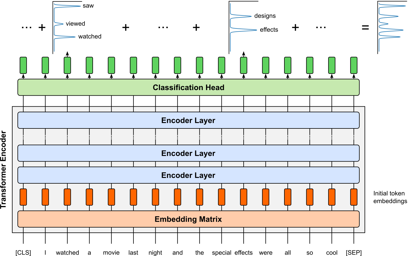
In general, the probability distributions are not sparse vectors as the probabilities for most words are greater than $0$, even if they are very small. SPLADE enforces sparsity explicitly through its training objective, rather than relying on architectural constraints alone. The model achieves high sparsity — often with over 99% of the vector dimensions being zero — through three primary mechanisms:
ReLU activation (the initial "zero-out"): SPLADE applies the Rectified Linear Unit (ReLU) function to the logits. Thus, any word that the model predicts as having a negative importance score is immediately set to exactly zero. Since most words in a $30k$-word vocabulary are irrelevant to a specific input sentence, ReLU "kills" the vast majority of these dimensions.
Log-saturation effect: After ReLU, SPLADE aggregates the scores from all input words to create a final document or query vector. It uses a logarithmic transformation. The logarithm prevents any single term from having an excessively high weight. In the context of sparsity, this "flattens" the distribution of scores. When combined with training losses (see next), it makes it easier for the model to push unimportant terms down to zero rather than letting them linger at low positive values.
Sparsity regularization (FLOPS loss): While ReLU and log-saturation provide the structural potential for sparsity, the model is explicitly trained to be sparse using a regularization term added to the main ranking loss. The most common loss used is the FLOPS (Floating Point Operations) loss. It minimizes the squared sum of the average weights across a batch of documents. This loss penalizes the model for "activating" too many tokens. It forces the model to be selective, ensuring that only the most semantically relevant tokens (and their expansions) receive non-zero weights.
Using this approach SPLADE expands a text into a sparse set of weighted vocabulary terms that includes both original words and semantically related ones. This expansion is learned end-to-end, allowing the model to activate dimensions corresponding to synonyms, paraphrases, or closely related concepts. The resulting representation remains interpretable and efficient like classic sparse methods, while significantly improving recall in retrieval scenarios by reducing lexical mismatch. In this way, SPLADE combines the strengths of symbolic and neural approaches: sparse, explainable representations that nevertheless capture semantic relationships beyond the surface form of the text.
Beyond SPLADE. The success of sparse contextual embeddings such as SPLADE highlighted that sparsity and contextualization are not opposing design choices, but can in fact be combined to yield powerful text representations. By demonstrating that neural language models can produce sparse, high-dimensional vectors that retain semantic awareness while remaining compatible with inverted indexes, SPLADE bridged a long-standing gap between traditional lexical retrieval and dense neural embeddings. This combination delivered strong empirical gains — particularly in recall and robustness to vocabulary mismatch — while preserving interpretability and efficiency, two properties that are often lost in dense representations.
These advantages spurred renewed interest in sparse neural representations and motivated the development of a broad family of related methods. Subsequent approaches explored alternative ways of inducing sparsity, different training objectives, and varied mechanisms for term expansion and weighting, all aiming to balance semantic expressiveness with the practical benefits of sparse indexing. Collectively, this line of work reflects a shift toward hybrid retrieval models that blend symbolic and neural signals, building on the insight that sparse contextual embeddings can serve as a unifying framework rather than a niche alternative to dense embeddings. While we omit a more detailed discussion of alternative methods, here is overview to selected alternatives:
- Context-Aware Sentence/Passage Term Importance Estimation For First Stage Retrieval (Dai et al., 2019)
- SparTerm: Learning Term-based Sparse Representation for Fast Text Retrieval (Bai et al., 2020)
- SPARTA: Efficient Open-Domain Question Answering via Sparse Transformer Matching Retrieval (Zhao et al., 2020)
- SPLADE v2: Sparse Lexical and Expansion Model for Information Retrieval (Formal et al., 2021)
- COIL: Revisit Exact Lexical Match in Information Retrieval with Contextualized Inverted List (Gao et al., 2021)
Dense Text Embeddings
Aggregation for Word Embeddings
A basic and widely used approach to generate text embeddings for sentences or documents is to aggregate the embeddings of the individual words that appear in the text. This idea naturally extends from word-level representations to text-level representations and can be applied to both static word embeddings**, such as Word2Vec, GloVe, or fastText, where each word has a single vector, and contextual word embeddings, such as those produced by ELMo or BERT, where each token embedding already incorporates information from its surrounding context.
In its simplest form, this aggregation is performed by averaging the word embedding vectors, resulting in a single fixed-length representation regardless of text length. An alternative approach to aggregate word embeddings can be implemented using different pooling strategies, most commonly mean pooling, but also max pooling or sum pooling over the token embeddings. When applied to contextual models like BERT, pooling is typically performed over the hidden states of the tokens in the sequence, rather than relying on a single special token representation. While these simple aggregation-based methods ignore higher-level compositional structure, they provide an efficient and surprisingly strong baseline for many tasks, and they form the conceptual foundation for more advanced sentence and document embedding techniques.
Simply averaging word embeddings treats all words as equally informative, which is rarely the case in natural language. Very frequent function words such as "the", "is", or "of" appear in almost every sentence and therefore dominate the aggregated representation, even though they contribute little to the semantic meaning of the text. As a result, naive averaging tends to blur distinctions between sentences and documents, producing embeddings that are overly influenced by global frequency patterns rather than by content-bearing words. Introducing additional steps such as smoothing or weighting before aggregation helps mitigate this problem by explicitly accounting for word importance. By down-weighting frequent words and relatively emphasizing rarer, more informative terms, the aggregated embedding better reflects the semantic content of the text. This often leads to more discriminative and stable text embeddings, forming a principled bridge between simple averaging methods and more sophisticated neural sentence embedding models.
Doc2Vec
Doc2Vec (Le and Mikolov, 2014) is a natural extension of the Word2Vec framework designed to learn fixed-length vector representations for larger pieces of text such as sentences, paragraphs, or entire documents, rather than just individual words. While Word2Vec captures semantic relationships at the word level by learning embeddings from local word co-occurrence patterns, it does not directly provide a single embedding that represents a whole text. Doc2Vec addresses this limitation by introducing an explicit document-level representation that complements word embeddings, enabling the model to capture the overall semantic meaning of longer texts in a compact vector form.
Conceptually, Doc2Vec follows the same distributional learning principle as Word2Vec (i.e., texts with similar contexts should have similar embeddings) but augments the training objective with a document identifier. This document vector acts as a shared memory that represents the topic or global semantics of the text and is learned jointly with word embeddings during training. As a result, Doc2Vec produces dense, low-dimensional text embeddings that can be directly used for downstream tasks such as document classification, clustering, and semantic search, making it a foundational method for document-level representation learning in NLP. Like Word2Vec, Doc2Vec is not a single method but comes in two main variants: PV-DM (Distributed Memory Model of Paragraph Vectors) and PV-DBOW (Distributed Bag-of-Words version of Paragraph Vectors).
PV-DM. The Distributed Memory Model of Paragraph Vectors (PV-DM) can be seen as a direct extension of the Continuous Bag-of-Words (CBOW) model from Word2Vec. PV-DM augments this setup by introducing a paragraph (or document) vector that represents the entire text segment. This paragraph vector serves as a persistent memory that captures the global semantics or topic of the paragraph, complementing the local contextual information provided by the surrounding words. More technically, PV-DM adds an additional embedding matrix $\mathbf{D}$ that maps each paragraph id to a single dense vector representation. This paragraph vector is then combined (e.g., by concatenation or averaging) with the embeddings vectors of the context words to predict the center word. The figure below illustrates this idea.
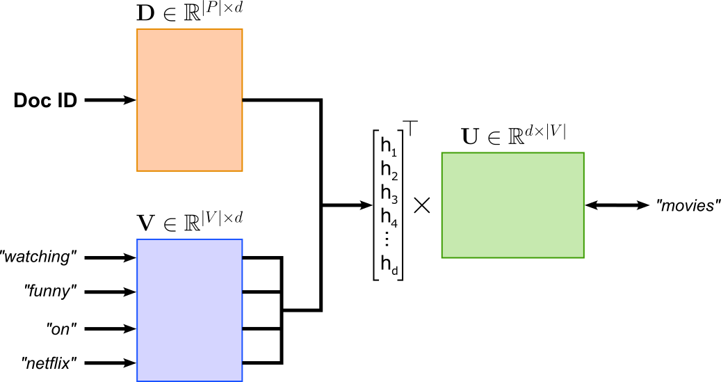
During training, both the word embeddings and the paragraph embeddings are learned jointly through this prediction task. By conditioning word predictions on a shared paragraph-level representation, PV-DM produces vector representation for each document in the training data. To generate vector representations for unseen documents, PV-DM uses an "inference stage" that treats the new document as a mini-training session. To this end, PV-DM initializes a new document vector (usually randomly) and then optimizes only this vector while keeping all word vectors fixed. The model runs a few iterations of gradient descent to adjust the document vector so that it is good at predicting the words in the document under the same objective used during training. Intuitively, this process finds the document vector that best explains the observed words given the learned word semantics. Although this inference step is slower than a single forward pass in modern encoder models, it allows Doc2Vec to assign meaningful embeddings to arbitrary new documents without retraining the entire model.
PV-DBOW. The Distributed Bag-of-Words version of Paragraph Vectors (PV-DBOW) extends ideas from the Skip-gram model to the paragraph level. While Skip-gram learns word embeddings by predicting surrounding context words from a center word, PV-DM uses the paragraph (or document) vector to predict randomly sampled words from the paragraph; see the figure below showing the basic setup.
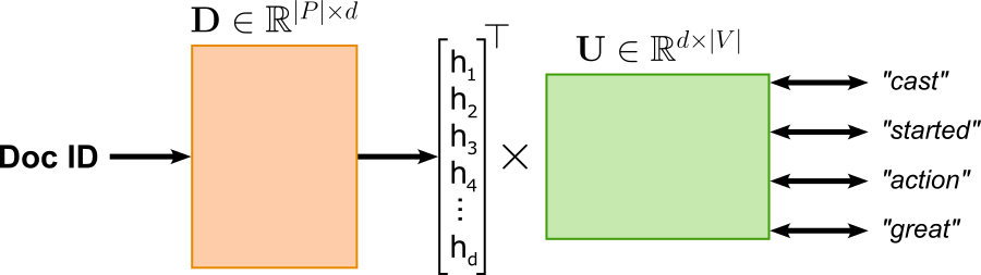
The PV-DBOW model is computationally more efficient and memory-friendly because it does not rely on input-side word embeddings during training. Unlike PV-DM, which must store and repeatedly access embeddings for context words (similar to CBOW), PV-DBOW uses only a paragraph vector to predict words sampled from the document. As a result, the model avoids combining multiple word vectors for each training instance, leading to fewer vector lookups and simpler computations per update, which directly translates into faster training. But like the PV-DM model, PV-DBOW also learns only vector representations for all paragraphs (or documents) in the training corpus. Thus, for unseen documents, the model randomly initializes and embedding vector for the document and performs a mini-training session to update this vector but keeping all other model parameters frozen.
Skip-Thought
Skip-Thought (Kiros et al., 2015) is motivated by the same core intuition as the Skip-gram model: linguistic units that appear in similar contexts should have similar representations. While Skip-gram operates at the word level, learning word embeddings by predicting surrounding words given a center word, Skip-Thought lifts this idea to the sentence level. Instead of treating words as the basic unit of meaning, Skip-Thought treats entire sentences as atomic units whose representations should capture the information needed to explain their neighboring context.
Concretely, Skip-Thought learns a sentence embedding by training a model to predict the preceding and subsequent sentence given an input sentence, rather than predicting nearby words. By requiring the embedding of a sentence to be informative enough to reconstruct its neighboring sentences, the model is encouraged to encode semantic content, syntax, and discourse-level information. In this way, Skip-Thought generalizes the Skip-gram objective from local word contexts to broader sentence contexts, providing a natural unsupervised framework for learning distributed sentence representations from raw text.
Skip-Thought is built around an encoder-decoder architecture that explicitly separates sentence representation from sentence generation. The encoder processes the input sentence (typically using an RNN) and compresses it into a single fixed-length vector that serves as the sentence embedding. The resulting sentence embedding is then used to condition one or more decoders, whose task is to generate the surrounding sentences in the original text. Given the embedding of the center sentence, the decoder predicts the words of the preceding and subsequent sentences, usually in an autoregressive manner. By training the model to reconstruct neighboring sentences from this single vector, Skip-Thought forces the encoder to produce embeddings that are informative about the broader discourse context in which the sentence appears.
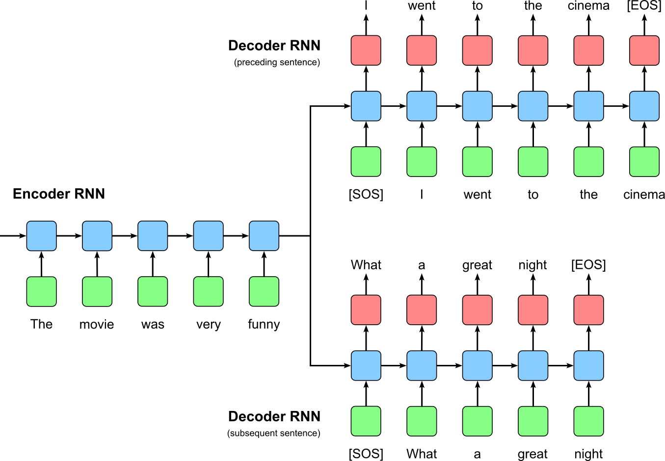
In the original architecture proposed by Kiros et al. (2015), as shown above, Skip-Thought uses two separate, independent decoders: one decoder is trained to generate the preceding sentence, the other decoder is trained to generate the subsequent sentence — but both decoders are conditioned on the same sentence embedding produced by the encoder. The main motivation for using different decoders is that the tasks of predicting the preceding and the subsequent sentence are not symmetric and therefore benefit from separate parameterizations. Language has a strong directional structure: the sentence that comes before a given sentence often serves a different discourse role (e.g., introducing context, setting up entities or topics) than the sentence that follows it (e.g., elaborating, explaining consequences, or continuing a narrative). A single shared decoder would be forced to model both distributions simultaneously, potentially blurring these distinct patterns.
SBERT (Sentence-BERT)
SBERT (Sentence-BERT) (Reimers and Gurevych, 2019) is a modification of the BERT architecture designed to produce semantically meaningful fixed-size embeddings for sentences and short texts. While BERT excels at generating contextualized token representations, it was not originally trained to yield sentence-level embeddings that can be compared directly using similarity measures such as cosine similarity. As a result, naive approaches, such as using the [CLS] token or averaging token embeddings, often perform suboptimally for tasks like semantic similarity, clustering, or retrieval.
SBERT extends BERT by placing it in a siamese or triplet network architecture and training it with sentence-level objectives. The basic concept of such architectures is to learn embeddings such that similar inputs are close together in the embedding space, while dissimilar inputs are far apart. In a siamese network, two identical subnetworks with shared weights encode a pair of inputs, and the model is trained with a loss that encourages the distance between embeddings to reflect their similarity (e.g., contrastive loss). A triplet network extends this idea by considering three inputs simultaneously: an anchor, a positive example (similar to the anchor), and a negative example (dissimilar to the anchor). The training objective enforces that the anchor's embedding is closer to the positive than to the negative by a margin.
In SBERT, the subnetwork is, of course, the BERT architecture, i.e., a transformer encoder, plus a pooling layer to aggregate all word embeddings into a single vector representing the input sentence. During training, multiple sentences are encoded independently using shared BERT weights, and the resulting embeddings are optimized so that semantically similar sentences are close in the embedding space while dissimilar ones are far apart. The optimization can be done using different objective functions (i.e., loss functions) depending on the nature of the training dataset:
Classification objective function: When training SBERT using a Natural Language Inference (NLI) dataset, the model leverages the sentence-level labels (entailment, contradiction, or neutral) to learn embeddings that capture semantic relationships between sentences. Each training example consists of a premise and a hypothesis. Both sentences are first encoded independently by the shared BERT encoder into fixed-length embeddings. These embeddings are then combined into a single representation for the pair. This combined vector is fed into a classification layer, often a simple feed-forward neural network, which predicts the NLI label. The original BERT paper proposes the following function to compute the output:
where $\mathbf{e}_A$ and $\mathbf{e}_B$ represent the word embeddings of the two Sentences $A$ and $B$ as a result of pooling their respective word embeddings as output of the BERT mode. The classification objective is the standard cross-entropy loss $\mathcal{L}_{CE}$ over the three possible labels. By optimizing this objective, SBERT learns sentence embeddings that encode semantic similarity and relational meaning, making them useful for downstream tasks such as semantic textual similarity, clustering, and retrieval. We can visualize the training setup using the classification objective function as shown below.
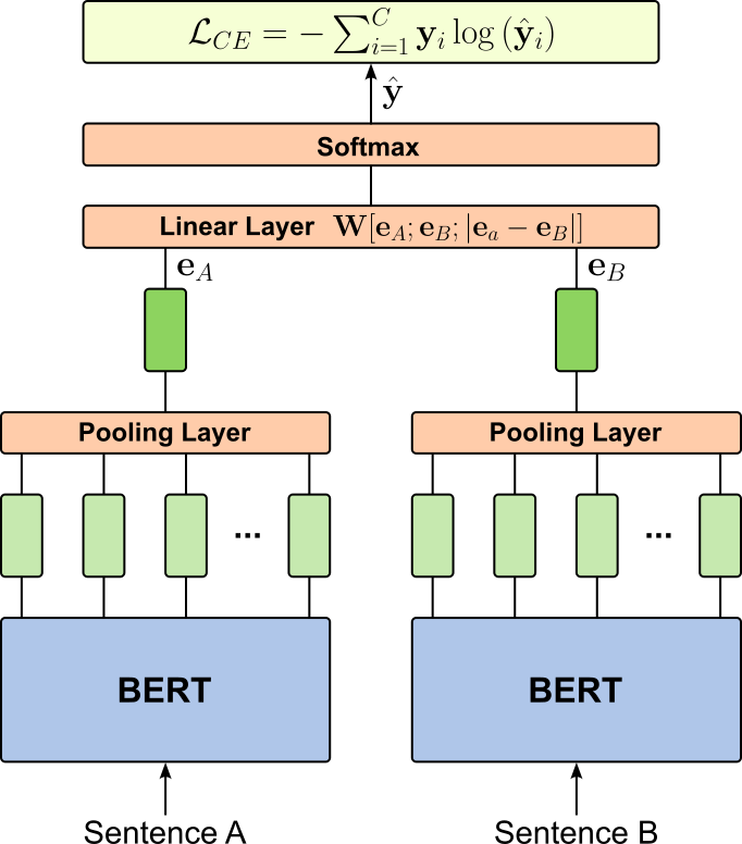
Regression objective function: When training SBERT on a Semantic Textual Similarity (STS) dataset, the goal is to produce embeddings such that the cosine similarity between two sentence embeddings reflects their human-annotated similarity score. Each training example consists of a pair of sentences along with a similarity score, usually normalized to the range $[0, 1]$. Both sentences are encoded independently using the shared BERT encoder, producing fixed-length embeddings. The similarity between the embeddings is then computed, commonly using cosine similarity, to serve as the model's prediction for the pair. The regression objective is typically the mean squared error (MSE) between the predicted similarity and the ground-truth similarity score. Formally, if $y_i$ is the true similarity and $\hat{y}_i$ is the cosine similarity of the embeddings for the $i$-th pair, the loss across all sentence pairs is:
Minimizing this loss encourages the model to position semantically similar sentences close together in the embedding space and dissimilar sentences further apart. By directly optimizing for similarity scores, SBERT learns embeddings that are well-aligned with human judgments of semantic similarity, making them highly effective for tasks such as semantic search, clustering, and retrieval. The figure below illustrates the overall training setup using the regression objective function — note that the MSE loss $\mathcal{L}_\text{MSE}$ in the figures refers to the loss with respect to a single sentence pair.
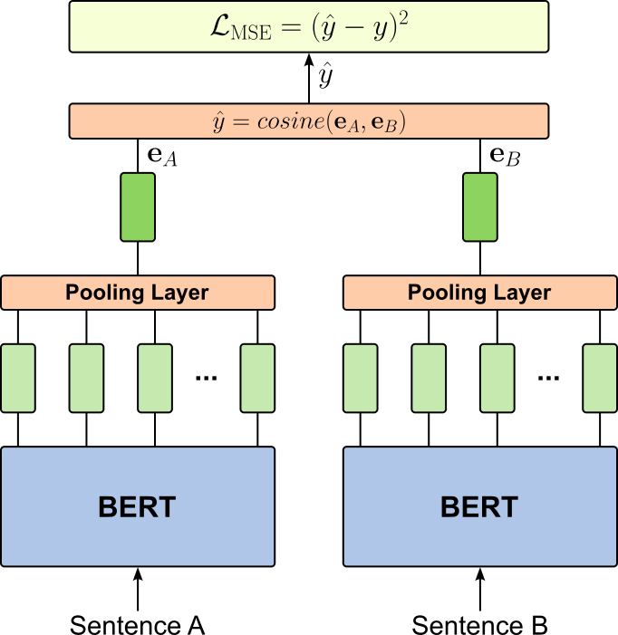
Triplet objective function: When training SBERT with a triplet objective, the goal is to directly shape the embedding space so that semantically similar sentences are closer to each other than to dissimilar sentences by a specified margin. Each training example is a triplet consisting of an anchor sentence, a positive sentence (semantically similar to the anchor), and a negative sentence (semantically dissimilar). The embeddings of these sentences are computed using the shared BERT encoder, and the model is trained to ensure that the distance between the anchor and positive embeddings is smaller than the distance between the anchor and negative embeddings by at least a margin $\alpha$. The typical triplet loss function is:
where $d(\mathbf{e}_{ref}, \mathbf{e}_{pos})$ and $d(\mathbf{e}_{ref}, \mathbf{e}_{neg})$ are distances (often cosine or Euclidean) between the anchor-positive and anchor-negative embeddings, respectively, and $\alpha$ is the margin hyperparameter. The loss is zero when the positive is closer to the anchor than the negative by at least $\alpha$, and otherwise it penalizes violations. Triplet training is often applied to datasets derived from semantic similarity or paraphrase corpora, such as STS datasets, Quora Question Pairs, or automatically mined paraphrase collections, where positive and negative examples can be reliably identified. This objective encourages the embedding space to reflect semantic relationships more directly than classification or regression losses. Like before, we can visualize the training setup, now using the triplet loss.

At inference time, SBERT produces fixed-length sentence embeddings via pooling over token embeddings, enabling efficient similarity computation and large-scale semantic search without requiring expensive cross-encoder comparisons.
Beyond SBERT. Text embeddings are a fundamental building block for many NLP and information retrieval tasks, as they provide a compact, numerical representation of text that enables semantic comparison, clustering, classification, and search. Most state-of-the-art text embedding methods today are based on the Transformer architecture, which excels at modeling contextual and long-range dependencies in language. Text embeddings remain a highly active and rapidly evolving area of research, and here is a list of some popular methods:
- Universal Language Model Fine-tuning for Text Classification (Howard and Ruder, 2018)
- Universal Sentence Encoder for English (Cer et al., 2019)
- Sentence-T5: Scalable Sentence Encoders from Pre-trained Text-to-Text Models (Ni et al., 2021)
- Text Embeddings by Weakly-Supervised Contrastive Pre-training (Wang et al., 2023)
- Towards General Text Embeddings with Multi-stage Contrastive Learning (Li et al., 2023)
- Qwen3 Embedding: Advancing Text Embedding and Reranking Through Foundation Models (Zhang et al., 2025)
- KaLM-Embedding: Superior Training Data Brings A Stronger Embedding Model (Hu et al., 2025)
- Gemini Embedding: Generalizable Embeddings from Gemini (Lee et al., 2025)
- Llama-Embed-Nemotron-8B: A Universal Text Embedding Model for Multilingual and Cross-Lingual Tasks (Babakhin et al., 2025)
In addition to academic research, many companies and institutions release text embedding models as part of commercial products or public APIs without fully disclosing the underlying architectures, training data, or optimization strategies. While these models often achieve strong empirical performance, the lack of detailed technical documentation or peer-reviewed publications makes it difficult to understand how the embeddings are constructed or to reproduce their results. This trend highlights a growing gap between state-of-the-art industrial systems and transparent, open research in text representation learning.
Consideration: Contextual Text Embeddings
As mentioned at the beginning, most common text embedding methods are static and return the same vector representation for the same input (i.e., sentence, paragraph, or document) as this input represents the whole context. However, it is often possible to "re-purpose" basic text embedding models to generate contextual embedding vectors by considering granularity levels.
A common example is to take a model that takes in paragraphs as input but returns multiple embedding vectors for each sentence in the paragraph. This is particularly easy to implement for any method that generates text embeddings by summing, averaging, or pooling word embeddings. In other words, instead of aggregating all word embeddings, we aggregate only the ones from the same sentence — sometimes called subsegment aggregation. Since the embedding vector of a word in a sentence depends on all words of the paragraph, now the sentence embedding also depends on the surrounding context. Thus, the same sentence used in a different paragraph will generally yield a different embedding vector.
Summary
Word and text embeddings have become a cornerstone of modern natural language processing because they provide a way to convert raw textual data into numerical representations that machine learning models, particularly neural networks, can process effectively. Text by itself is inherently symbolic and discrete, making it incompatible with operations such as matrix multiplication and gradient-based optimization that underlie most neural architectures. Embeddings solve this problem by mapping words, sentences, paragraphs, or entire documents to vectors in a continuous space, where semantic relationships are often preserved. This transformation allows models to reason about text in a mathematically meaningful way, supporting tasks from classification and sentiment analysis to retrieval and language generation.
Embeddings come with different characteristics that determine their suitability for specific tasks. One key distinction is granularity: word embeddings represent individual tokens, capturing local semantic information, while text embeddings summarize larger units such as sentences, paragraphs, or documents, integrating information across multiple words. Another important property is sparsity: sparse embeddings, such as traditional bag-of-words or modern methods like SPLADE, represent text with high-dimensional vectors where most values are zero, allowing for efficient indexing and interpretability. Dense embeddings, by contrast, compress information into lower-dimensional vectors, providing richer semantic representations at the cost of higher computational complexity. Finally, embeddings can be static or contextual: static embeddings assign the same vector to a word or text regardless of its usage, whereas contextual embeddings produce different vectors depending on surrounding words, sentence structure, or even task-specific signals, capturing polysemy and fine-grained meaning.
The strategies for generating embeddings are diverse and continually evolving. Early methods like Word2Vec, GloVe, and fastText focused on static word-level embeddings learned from co-occurrence statistics or predictive objectives. Later approaches, such as ELMo, BERT, and SBERT, introduced contextualized embeddings, enabling models to represent words and sentences differently depending on the input context. Sparse contextual embeddings like SPLADE combine the interpretability and efficiency of sparse representations with the semantic richness of neural language models. Aggregation techniques, hierarchical models, and task-specific adaptations further expand the range of approaches for encoding longer texts and documents.
Embedding research remains an active and highly impactful area of study because high-quality embeddings underpin many downstream applications. They are crucial in retrieval-augmented generation (RAG) systems, semantic search engines, recommendation systems, and clustering pipelines, where embedding quality directly affects the relevance and accuracy of results. Advances in embedding techniques continue to improve the ability of models to understand and manipulate language efficiently, balancing trade-offs between expressiveness, interpretability, computational cost, and suitability for specific tasks. This ongoing innovation underscores why embeddings are both a foundational and rapidly evolving component of modern NLP.